Draw From The BART Prior
samplePriorPredictive.RdDraws repeatedly from the prior a dbartsSampler runs under - the
hyperparameters that carry a prior, tree structure, leaf values, and optionally the observation
model - and evaluates the resulting forest at x.test.
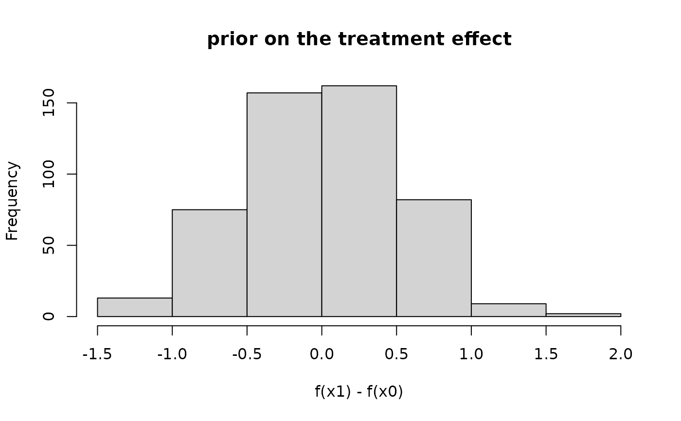
Useful for calibrating priors before ever fitting to data, e.g. inspecting the implied prior on a
treatment effect \(f(x_1) - f(x_0)\). The sampler passed in is never modified.
Usage
samplePriorPredictive(
  sampler, x.test = NULL, n.samples = 200L,
  type = c("ev", "ppd"), offset.test = NULL,
  n.threads = sampler$control@n.threads
)
Arguments
- sampler
A
dbartsSampler. Left unmodified: the function operates on a freshly constructed private sampler, built from this sampler's control, model, and data, with its own engine state.- x.test
A matrix of predictors at which to evaluate the drawn forests, in the form accepted by
predict.NULL(the default) evaluates at the sampler's own training predictors.- n.samples
A positive integer giving the number of independent prior draws to return.
- type
"ev"draws \(E[y \mid x]\) under the prior, matching whatextractandpredictcall"ev": the forest sum on the response scale for a gaussian or Student-t sampler; the link-transformed probability for a probit or logistic one; the mean count \(\exp(\eta)\) for a negative-binomial one, the center andoffset.testinside \(\eta\); the \(K\) category probabilities for an ordinal or multinomial one."ppd"adds the observation model on top: gaussian noise with sigma freshly drawn from its own prior for each sample; for Student-t, sigma times \(t_\nu\) noise at the family's df, or at the sample's df drawn from its prior when the df is estimated; a bernoulli draw from the"ev"probabilities for a binary sampler, a binomial one included, one trial per row aspredictdraws at a new row given no weights; a negative-binomial count at the sample's shape, fixed or drawn; an integer category code \(1, \ldots, K\) for an ordinal sampler, and for a multinomial one whose response was written as a factor; a count vector of one trial for a multinomial sampler whose response was written as a count matrix, whatever the rows' trials, aspredictdraws at a new row. A$setResponse, which on a multinomial sampler takes a count matrix, makes the response one written as a count matrix. On an aft (survival) sampler the draw is on the log-time scale (the model fits \(\log T\)), and on a heteroscedastic one the noise is drawn at a prior draw of that observation's own \(s(x)\) rather than at a scalar sigma. Unlikeextract's posterior"ppd", prior predictive draws are weight-blind: they use unit weights rather than a weighted precision (\(\sigma / \sqrt{w}\) for gaussian), and a row of weight 0 is drawn as every other row is, where the posterior draw at it isNA; each draw is one observation, as a training row's posterior draw is under every reading. Supply any weighted precision downstream.- offset.test
A numeric offset added to the forest sum, as in
predict; recycled to the number of rows ofx.testif of length 1, orNULL(the default) for none. On a multinomial sampler it ispredict's matrix of category offsets, one row per row ofx.testand one column per category; a sampler carrying a category offset requires it (an all-zero matrix for the offset-free surface).- n.threads
Forwarded to the underlying
predictcalls.
Details
Each of the n.samples draws independently redraws the hyperparameters, every tree's
structure (sampleTreesFromPrior) and leaf values (sampleLeafParametersFromPrior)
from scratch, then evaluates the resulting forest at x.test - there is no MCMC dependence
between rows of the result, unlike a posterior sample from run.
The hyperparameters drawn are those the sampler draws: \(k\) from its chi()
hyperprior (which normal(sd = invchi()) is), a Student-t df from its prior on the
family's grid when the df is estimated, a negative-binomial shape from its prior on its grid when
the shape is estimated, and an ordinal sampler's cutpoints (the first at 0, each gap log-normal),
one set per sample shared by every row. A fixed \(k\), df or shape is used as it stands.
An improper leaf prior, invchi() with scale 0 or chi() with an infinite scale, has
no prior draws and is refused.
Under split.probs = dart() the prior the sampler runs is not the stated Dirichlet on the
split probabilities alone: the sampler never holds a tree with an empty leaf, so its prior on the
split probabilities and the trees together is the stated one restricted to forests in which no
tree has an empty leaf. Each sample draws the concentration and the split probabilities from the
stated prior and every tree from the tree prior given them, and redraws the whole, split
probabilities included, while any tree has an empty leaf, with no limit on the attempts, so
every sample is an exact draw of that prior. How often a whole draw is kept falls with the number
of trees and rises with the number of rows: about one in a hundred at 60 rows, 8 columns and 200
trees, where 1,000 samples take a few seconds. With few rows and many trees the draw can take
long: at 8 columns, 1,000 samples take about a minute at 60 rows and 500 trees, and one and a
half to two and a half hours at 60 rows and 1,000 trees or at 30 rows and 500 trees. Once the
attempts made project a call longer than about a minute, a warning, printed when issued, gives the
share of draws kept so far and the projected time. The draw can be interrupted as a run is; the
sampler passed in is left as it was.
For type = "ppd" on a gaussian sampler, sigma is drawn once per sample from the model's
residual-variance prior: a scaled-inverse-chi-squared calibrated so that
\(P(\sigma < \code{sigest}) = \code{quant}\) when the prior is
chisq (see dbartsPriors), or the sampler's fixed value when the prior is
fixed.
A heteroscedastic sampler (dbarts's variance) has no single sigma to draw,
so the noise is its own surface: each sample additionally redraws the variance forest from its
prior (sampleVarianceForestFromPrior) and adds \(s(x)\epsilon\) at the rows
being predicted, \(s^2(x)\) read there through
getVariance. The mean draws, and every type = "ev"
draw, are unaffected.
Prior draws are chain-free: the private sampler runs one chain whatever sampler's
n.chains, since there is no mixing or convergence concept for draws that are already
independent by construction.
Seeding follows from the private sampler being constructed fresh on every call. When the
control's seed is NULL (the default), the engine RNG
is seeded from R's random number stream at construction, so successive calls return independent
draws, and a set.seed beforehand makes the whole draw - forests and observation
layer alike - reproducible. When the control fixes seed, the engine stream is pinned:
every call replays the identical sequence of hyperparameters and forests, with only the R-side
"ppd" observation layer (sigma, the noise, counts and categories) still governed by
set.seed.
To compare the prior at two or more covariate settings with paired forests - as for a treatment
effect - stack the settings as rows of a single x.test and difference the corresponding
columns of the result; see ‘Examples’. Two separate calls draw independent sets of forests
(unless seed is fixed, as above) and so cannot be differenced meaningfully.
Value
A matrix with n.samples rows and one column per row of x.test (or of the training
predictors, when x.test is NULL) - the combined-draws convention extract
uses for a single chain, with no chain dimension. For an ordinal or multinomial sampler
"ev" is an n.samples by rows by \(K\) array of category probabilities, as is
"ppd" on a multinomial sampler whose response was written as a count matrix, holding the counts; category codes
are integers.
See also
dbartsSampler for sampleTreesFromPrior, sampleLeafParametersFromPrior,
and predict, the building blocks this function composes. dbarts for
creating a sampler. extract for the same "ev"/"ppd" vocabulary applied to
posterior draws.
Examples
n <- 100
x <- matrix(runif(n * 2), n, 2)
y <- x[, 1] - x[, 2] + rnorm(n, 0, 0.2)

sampler <- dbarts(y ~ x, control = dbartsControl(n.chains = 1L, n.threads = 1L))

## prior-predictive draws of a treatment effect f(x1) - f(x0), holding the
## other covariate fixed at its midpoint: calibrates the prior before ever
## touching y. Stacking both settings into one x.test pairs the forests, so
## the two columns of the result come from the same drawn function.
xContrast <- rbind(c(0, 0.5), c(1, 0.5))
colnames(xContrast) <- colnames(sampler$data@x)

f <- samplePriorPredictive(sampler, x.test = xContrast, n.samples = 500L)
effect <- f[, 2] - f[, 1]
hist(effect, main = "prior on the treatment effect", xlab = "f(x1) - f(x0)")