Working with dbarts Saved Trees
Vincent Dorie
2026-07-25
Source:vignettes/working_with_saved_trees.Rmd
working_with_saved_trees.RmdWhen a dbarts model is fit with the
keepTrees option set to TRUE, the sampler will
return those trees in a “flat” format that corresponds to a depth-first,
left-hand traversal. Recursion can be used to map functions over the
nodes in this structure, aggregating statistics of interest.
Simulation
To illustrate, we generate a fake dataset according to the “Friedman 1” model (Friedman 1991).
Model Fitting
In order to interrogate the trees, they must be saved when the model is fit. This is accomplished by setting:
- For
bartBT:keeptrees = TRUE - For
bart:keepTrees = TRUE - For a custom
dbartsSampler,control = dbartsControl(keepTrees = TRUE)
In the context of our fake data, with small sample numbers for illustrative purposes, a model can be fit thusly:
## dbarts: 'bart' is the modern front door (formerly 'bart2'); 'bartBT' is the BayesTree-style one, with 0.9-x's argument names and defaults. A BayesTree-spelled 'bart' call is forwarded to 'bartBT' with a warning for this release.
bartFit <- bart(
    y ~ ., data,
    n.samples = 4,   # number of posterior samples
    n.burn = 1000,   # number of "warmup" samples to discard
    n.chains = 2,    # number of independent, parallel chains
    n.threads = 1,   # units of parallel execution
    n.trees = 3,     # number of trees per chain
    seed = 56,       # the first tree printed below has 7 nodes
    keepTrees = TRUE,
    verbose = FALSE)
Extracting Trees
The extract function accepts as a type the value
"trees". If present, the arguments chainNums,
sampleNums, and/or treeNums can be used to
extract only a subset of trees, and forest selects among a
fit’s forests (a single index, a vector, or the default of every forest)
on a fit with more than one, such as a Bayesian causal forest or a
multinomial fit itself. On such a fit the forest column of
the result is a factor whose levels are the forests’ labels, in forest
order (forest1, forest2 and so on for a forest
with none), so that trees$forest == "z" selects a forest
and as.integer(trees$forest) gives its position.
trees <- dbarts::extract(bartFit, "trees")Flattened Trees
The trees data frame corresponds to a depth-first,
left-hand-side tree traversal.
##    chain sample tree   n var       value
## 1      1      1    1 100   2  0.46454671
## 2      1      1    1  35   7  0.24853041
## 3      1      1    1   6  -1  0.04584981
## 4      1      1    1  29  -1 -0.02522418
## 5      1      1    1  65   5  0.26888559
## 6      1      1    1  15  -1  0.04883142
## 7      1      1    1  50  -1  0.17614013
## 8      1      1    2 100   4  0.25606734
## 9      1      1    2  32   3  0.93191654
## 10     1      1    2  31  -1 -0.11875045
The columns refer to:
-
forest,chain,sample,tree- index variables;forestis present only on a fit with more than one forest, so not on the single-forest fit above;chainis always present inextract(type = "trees"), 1 on a one-chain fit -
n- number of observations in node (from the training data, or fromnewdatawhen it is supplied; see “Counts for New Data” below) -
var- either the index of the variable used for splitting or -1 if the node is a leaf -
value- the cut point for an ordinal split (observations less than or equal to it go left);NAfor a categorical split (see “Categorical Splits” below); otherwise the leaf’s fitted value, which is its intercept under a linear leaf andNAunder a Gaussian-process leaf (its fit is a function of the leaf’s covariates rather than a scalar - seepredictfor those) -
directions- present when the sampler has any categorical predictor: for a categorical split, one"L"/"R"character per level in level order, giving the branch that level is sent down;NAfor ordinal splits and for leaves -
missing- present when any predictor has missing values:"L"/"R"giving the branch anNAon the split variable follows;NAwhere the rule has no missing values to route -
beta.<column>- one per covariate designated by alinearorgpleaf prior, holding that leaf’s coefficient;NAon internal nodes, absent entirely under the default constant leaf
The mapping between the values of var and the variable
names can be looked up in the internal copy of the data that the sampler
stores. This can be found in a fitted model as the element
fit$data@x, as seen below.
Categorical Splits
A categorical predictor’s rule sends a subset of its levels down each
branch rather than cutting at a threshold, so it cannot be summarized by
a single cut point: value is NA for these
rules, and the split instead appears in directions.
set.seed(77)
n.cat <- 60
g <- factor(sample(letters[1:4], n.cat, replace = TRUE))
y.cat <- ifelse(g %in% c("a", "b"), 5, -5) + rnorm(n.cat, 0, 0.5)

catFit <- bart(y ~ g, data.frame(y = y.cat, g = g),
               n.trees = 3L, n.samples = 1L, n.burn = 20L, n.chains = 1L,
               n.threads = 1L, keepTrees = TRUE, seed = 0, verbose = FALSE)
catTrees <- dbarts::extract(catFit, "trees")
print(subset(catTrees, var != -1))
## chain sample tree n var value directions
## 1 1 1 1 60 1 NA LLRR
## 5 1 1 3 60 1 NA LLRRg’s levels are "a", "b",
"c", "d", in that order, so the first tree’s
directions of "LLRR" sends a and
b left and c and d right;
plotTree labels the same rule with the levels its left
branch takes, "g in {a,b}".
Tree Traversal
A useful technique for processing trees is recursion. By having the function return the number of nodes it has processed, it is possible to advance from the left-hand-side to the right by skipping ahead the appropriate number of rows. For example:
# Turns a flattened tree data frame into a list of lists, or a "natural" tree
# structure.
rebuildTree <- function(tree, object) {
    # A linear leaf's beta.<column> columns ride along automatically; a
    # constant leaf has none.
    slopeColumns <- names(tree)[startsWith(names(tree), "beta.")]

    # Define a worker function that will be recursively called on every node.
    rebuildTreeRecurse <- function(tree) {
        node <- list(
            value = tree$value[1],
            n     = tree$n[1]
        )
        # Check node if is a leaf, and if so return early.
        if (tree$var[1] == -1) {
            if (length(slopeColumns) > 0) {
                node$beta <- unlist(tree[1, slopeColumns])
            }
            node$n_nodes <- 1
            return(node)
        }

        node$var <- variableNames[tree$var[1]]

        # By removing the current row, we can recurse down the left branch.
        headOfLeftBranch <- tree[-1,]
        left <- rebuildTreeRecurse(headOfLeftBranch)
        n_nodes.left <- left$n_nodes
        left$n_nodes <- NULL
        node$left <- left

        # The right branch is obtained by advancing past the left nodes.
        headOfRightBranch <- tree[seq.int(2 + n_nodes.left, nrow(tree)),]
        right <- rebuildTreeRecurse(headOfRightBranch)
        n_nodes.right <- right$n_nodes
        right$n_nodes <- NULL
        node$right <- right

        node$n_nodes <- 1L + n_nodes.left + n_nodes.right

        return(node)
    }
    variableNames <- colnames(object$fit$data@x)

    result <- rebuildTreeRecurse(tree)
    result$n_nodes <- NULL
    return(result)
}

treeOfInterest <- subset(trees, chain == 1 & sample == 3 & tree == 1)
print(rebuildTree(treeOfInterest, bartFit))
## $value
## [1] 0.4645467
##
## $n
## [1] 100
##
## $var
## [1] "X2"
##
## $left
## $left$value
## [1] 0.009059387
##
## $left$n
## [1] 35
##
##
## $right
## $right$value
## [1] 0.2688856
##
## $right$n
## [1] 65
##
## $right$var
## [1] "X5"
##
## $right$left
## $right$left$value
## [1] 0.06530634
##
## $right$left$n
## [1] 15
##
##
## $right$right
## $right$right$value
## [1] 0.1580289
##
## $right$right$n
## [1] 50Under a linear leaf prior, the same function attaches
each leaf’s slopes as $beta:
set.seed(21)
n.lin <- 60
x1.lin <- runif(n.lin); x2.lin <- runif(n.lin)
y.lin <- 3 * x1.lin + rnorm(n.lin, 0, 0.2)

linearFit <- dbarts(
    y.lin ~ x1.lin + x2.lin, data.frame(x1.lin, x2.lin, y.lin),
    leaf.prior = linear("x1.lin"),
    control = dbartsControl(n.chains = 1L, n.threads = 1L,
                            keepTrees = TRUE, n.samples = 2L, n.burn = 10L),
    n.trees = 3L)
invisible(linearFit$run())
linearTrees <- subset(linearFit$getTrees(), sample == 1 & tree == 1)
print(rebuildTree(linearTrees, list(fit = linearFit)))
## $value
## [1] 0.3726957
##
## $n
## [1] 60
##
## $var
## [1] "x1.lin"
##
## $left
## $left$value
## [1] 0.0758541
##
## $left$n
## [1] 20
##
## $left$beta
## [1] 0.343214
##
##
## $right
## $right$value
## [1] -0.04398386
##
## $right$n
## [1] 40
##
## $right$beta
## [1] 0.2875415Using a by statement, it is possible to “rebuild” all
trees at once:
Plotting Trees
dbartsSampler objects have a plotTree
method that can be used to visualize single trees:
bartFit$fit$plotTree(chainNum = 1, sampleNum = 3, treeNum = 1)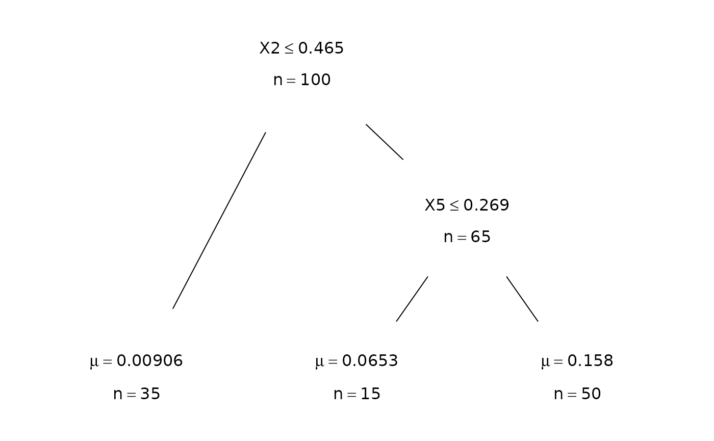
Getting Tree Predictions
The following function traverses a flattened tree, splits
observations while going down the branches, and populates a vector
giving the predicted value of that tree on input data. It requires data
in the same format as the fitted bart model so that it can evaluate the
splits. As written it assumes an ordinal split and a constant leaf; a
categorical split’s condition instead reads directions, and
a linear or gp leaf’s fitted value depends on the leaf’s covariates
rather than being a single number - use predict for
those.
getPredictionsForTree <- function(tree, x) {
    predictions <- rep(NA_real_, nrow(x))

    getPredictionsForTreeRecursive <- function(tree, indices) {
        if (tree$var[1] == -1) {
            # Assigns in the calling environment by using <<-
            predictions[indices] <<- tree$value[1]
            return(1)
        }

        goesLeft <- x[indices, tree$var[1]] <= tree$value[1]
        headOfLeftBranch <- tree[-1,]
        n_nodes.left <- getPredictionsForTreeRecursive(
            headOfLeftBranch, indices[goesLeft])

        headOfRightBranch <- tree[seq.int(2 + n_nodes.left, nrow(tree)),]
        n_nodes.right <- getPredictionsForTreeRecursive(
            headOfRightBranch, indices[!goesLeft])

        return(1 + n_nodes.left + n_nodes.right)
    }

    getPredictionsForTreeRecursive(tree, seq_len(nrow(x)))

    return(predictions)
}

getPredictionsForTree(treeOfInterest, bartFit$fit$data@x[1:5,])
## [1] 0.009059387 0.158028894 0.158028894 0.009059387 0.065306342A by statement can be used to obtain all predictions for
all trees.
Counts for New Data
The recursion above routes new data through the trees by hand. To
simply count how a new dataset distributes across the (frozen)
partition, pass newdata to extract: the tree
structure, split rules, and leaf predictions are unchanged, and only the
n column is recomputed by routing that data through each
tree. The predictors are supplied in the same form as for
predict.
newData <- data[1:5, ]
newTrees <- dbarts::extract(bartFit, "trees", newdata = newData, sampleNums = 3, treeNums = 1)
print(subset(newTrees, chain == 1))
## chain sample tree n var value
## 1 1 3 1 5 2 0.464546706
## 2 1 3 1 2 -1 0.009059387
## 3 1 3 1 3 5 0.268885592
## 4 1 3 1 1 -1 0.065306342
## 5 1 3 1 2 -1 0.158028894Advanced Traversal
The following function can be used to map an arbitrary function over a tree.
mapOverNodes <- function(tree, f, ...) {
    mapOverNodesRecurse <- function(tree, depth, f, ...) {
        node <- list(
            value = tree$value[1],
            n = tree$n[1],
            depth = depth
        )
        if (tree$var[1] == -1) {
            node$n_nodes <- 1
            node$f.x <- f(node, ...)
            return(node)
        }
        node$var <- tree$var[1]
        node$f.x <- f(node, ...)

        headOfLeftBranch <- tree[-1,]
        left <- mapOverNodesRecurse(headOfLeftBranch, depth + 1, f, ...)
        n_nodes.left <- left$n_nodes
        left$n_nodes <- NULL
        node$left <- left


        headOfRightBranch <- tree[seq.int(2 + n_nodes.left, nrow(tree)),]
        right <- mapOverNodesRecurse(headOfRightBranch, depth + 1, f, ...)
        n_nodes.right <- right$n_nodes
        right$n_nodes <- NULL
        node$right <- right

        node$n_nodes <- 1 + n_nodes.left + n_nodes.right
        return(node)
    }
    result <- mapOverNodesRecurse(tree, 1, f, ...)
    result$n_nodes <- NULL
    return(result)
}
As an example of its usage, the following function aggregates all ancestor/descendant relationships in a tree. In a data object - here an R environment - it keeps track of the current state of traversal. This includes the variables that have been used for splits above the current node and also includes the current node’s depth, which is used to detect backtracking.
observeInteractions <- function(node, ...) {
    if (is.null(node$var)) return(NULL)

    interactionData <- list(...)$interactionData
    # Make the current node visibile inside the environment.
    interactionData$node <- node
    with(interactionData, {
        if (node$depth <= currentDepth) {
            # If true, we have backtracked to go down the right branch, so we
            # remove the variables from the left branch.
            currentVariables <- currentVariables[seq_len(node$depth - 1)]
        }
        if (length(interactionData$currentVariables) > 0) {
            # This is a brute-force way of updating the following indices,
            # relying on the column-major storage order that R uses:
            #     hasInteraction[currentVariables,,drop = FALSE][,node$var]
            updateIndices <- currentVariables +
                (node$var - 1) * nrow(hasInteraction)
            hasInteraction[updateIndices] <- TRUE
        }
        currentVariables <- c(currentVariables, node$var)
        currentDepth <- node$depth
    })
    rm("node", envir = interactionData)

    # Since the function is used for its side effects, there isn't a return
    # value.
    return(NULL)
}

numVariables  <- ncol(bartFit$fit$data@x)
variableNames <- colnames(bartFit$fit$data@x)

# Define this as an environment as they are mutable
interactionData <- list2env(list(
    currentDepth = 0,
    currentVariables = integer(),
    hasInteraction = matrix(
        data = FALSE,
        ncol = numVariables, nrow = numVariables,
        dimnames = list(ancestor = variableNames, descendant = variableNames)
    )
))

invisible(mapOverNodes(
    treeOfInterest,
    observeInteractions,
    interactionData = interactionData
))
After execution, the boolean matrix in the interaction data environment will contain all ancestor/descendant relationships in this tree.
print(interactionData$hasInteraction)## descendant
## ancestor X1 X2 X3 X4 X5 X6 X7 X8 X9 X10
## X1 FALSE FALSE FALSE FALSE FALSE FALSE FALSE FALSE FALSE FALSE
## X2 FALSE FALSE FALSE FALSE TRUE FALSE FALSE FALSE FALSE FALSE
## X3 FALSE FALSE FALSE FALSE FALSE FALSE FALSE FALSE FALSE FALSE
## X4 FALSE FALSE FALSE FALSE FALSE FALSE FALSE FALSE FALSE FALSE
## X5 FALSE FALSE FALSE FALSE FALSE FALSE FALSE FALSE FALSE FALSE
## X6 FALSE FALSE FALSE FALSE FALSE FALSE FALSE FALSE FALSE FALSE
## X7 FALSE FALSE FALSE FALSE FALSE FALSE FALSE FALSE FALSE FALSE
## X8 FALSE FALSE FALSE FALSE FALSE FALSE FALSE FALSE FALSE FALSE
## X9 FALSE FALSE FALSE FALSE FALSE FALSE FALSE FALSE FALSE FALSE
## X10 FALSE FALSE FALSE FALSE FALSE FALSE FALSE FALSE FALSE FALSEFinally, the entire process can be wrapped in a by
statement and the results aggregated across all trees in order to count
the number of times variables have specific relationships.