Building a Gibbs Sampler with dbarts
Vincent Dorie
2026-08-19
Source:vignettes/gibbs_sampler_mixture_model.Rmd
gibbs_sampler_mixture_model.RmdFor users who are comfortable with writing their own posterior
samplers, dbarts makes it easy to incorporate a linear BART
component in a Gibbs sampler. In the example below, we fit a functional
mixture model, where observations may have come from one of two
underlying functions and class membership is unobserved.
Model
Performing inference conditional on , we assume that:
and that is unobserved. To make the model fully Bayesian, we impose a prior on . and have implicit priors defined by BART.
Conditional Posteriors
To implement a Gibbs sampler, we will have to produce updates for and . After writing down the joint distribution of , , , , and , we have:
where is the density of a normal distribution. This yields an overall strategy of:
- Draw a sample from BART
- Draw samples of and
- Draw a sample of
- Use , , and to draw a sample of
- Use to draw a sample of
Simulated Data
To illustrate, we create some toy data. The simulated data is visualized later, together with the fitted model.
# Underlying functions
f0 <- function(x) 90 + exp(0.06 * x)
f1 <- function(x) 72 + 3 * sqrt(x)

set.seed(2793)

# Generate true values.
n <- 120
p.0 <- 0.5

z.0 <- rbinom(n, 1, p.0)
n1 <- sum(z.0); n0 <- n - n1

# In order to make the problem more interesting, x is confounded with both
# y and z.
x <- numeric(n)
x[z.0 == 0] <- rnorm(n0, 20, 10)
x[z.0 == 1] <- rnorm(n1, 40, 10)
y <- numeric(n)
y[z.0 == 0] <- f0(x[z.0 == 0])
y[z.0 == 1] <- f1(x[z.0 == 1])
y <- y + rnorm(n)

data_train <- data.frame(y = y, x = x, z =     z.0)
data_test  <- data.frame(       x = x, z = 1 - z.0)
Implementing a Gibbs Sampler
For this specific model, the sampler needs to be updated with new
predictor variables/covariates. This can be done with a
dbartsSampler reference class object by calling the
sampler$setPredictor function. As, given any
,
the sampler also needs to evaluate
,
we utilize the test slot of the sampler and keep it up-to-date with the
“counterfactual” predictor using the
sampler$setTestPredictor function. Models that instead
modify the response variable can use the
sampler$setResponse or sampler$setOffset
functions.
One complication in updating the predictor matrix while the sampler
runs is that new values of
must leave the sampler in an internally consistent state. During warmup
this constraint is ignored; after warmup is complete, rejection sampling
is used to guarantee that no leaf nodes are empty. This is accomplished
by using the forceUpdate argument to
setPredictor and checking that the logical response is
TRUE.
n_warmup  <- 100
n_samples <- 500
n_total   <- n_warmup + n_samples

# Allocate storage for result.
samples_p   <- rep.int(NA_real_, n_samples)
samples_z   <- matrix(NA_real_, n_samples, n)
samples_mu0 <- matrix(NA_real_, n_samples, n)
samples_mu1 <- matrix(NA_real_, n_samples, n)

library(dbarts, quietly = TRUE)
## dbarts: 'bart' is the modern front door (formerly 'bart2'); 'bartBT' is the BayesTree-style one, with 0.9-x's argument names and defaults. A BayesTree-spelled 'bart' call is forwarded to 'bartBT' with a warning for this release.
# We only need to draw one sample at a time, although for illustrative purposes
# a small degree of thinning is done to the BART component.
control <- dbartsControl(updateState = FALSE, verbose = FALSE,
                         n.burn = 0L, n.samples = 1L, n.thin = 3L,
                         n.chains = 1L)
# We create the sampler with a z vector that contains at least one 1 and one 0,
# so that all of the cut points are set correctly.
sampler <- dbarts(y ~ x + z, data_train, data_test, control = control)

# Sample from prior.
p <- rbeta(1, 1, 1)
z <- rbinom(n, 1, p)

# Ignore result of this sampler call
invisible(sampler$setPredictor(x = z, column = 2, forceUpdate = TRUE))
sampler$setTestPredictor(x = 1 - z, column = 2)
sampler$sampleTreesFromPrior()

for (i in seq_len(n_total)) {
  # Draw a single sample from the posterior of f and sigma^2.
  samples <- sampler$run()

  # Recover f(x, 1) and f(x, 0).
  mu0 <- ifelse(z == 0, samples$train[,1], samples$test[,1])
  mu1 <- ifelse(z == 1, samples$train[,1], samples$test[,1])

  p0 <- dnorm(y, mu0, samples$sigma[1]) * (1 - p)
  p1 <- dnorm(y, mu1, samples$sigma[1]) * p
  p.z <- p1 / (p0 + p1)
  z <- rbinom(n, 1, p.z)

  if (i <= n_warmup) {
    sampler$setPredictor(x = z, column = 2, forceUpdate = TRUE)
  } else while (sampler$setPredictor(x = z, column = 2) == FALSE) {
    z <- rbinom(n, 1, p.z)
  }
  sampler$setTestPredictor(x = 1 - z, column = 2)

  n1 <- sum(z); n0 <- n - n1
  p <- rbeta(1, 1 + n1, 1 + n0)

  # Store samples if no longer warming up.
  if (i > n_warmup) {
    offset <- i - n_warmup
    samples_p[offset] <- p
    samples_z[offset,] <- z
    samples_mu0[offset,] <- mu0
    samples_mu1[offset,] <- mu1
  }
}
Saveing the sampler
To use save and load on the sampler, it
must first be told to write its state out as an R
object:
sampler$storeState()Visualizing the Result
Finally, we visualize the results. In the graph below, the estimated label of observations encircles the true labels, both of which are represented by point color. We see that, beyond the range of the observed data, the estimated functions regress towards each other and points start to be mislabeled.
mean_mu0 <- apply(samples_mu0, 2, mean)
mean_mu1 <- apply(samples_mu1, 2, mean)

ub_mu0 <- apply(samples_mu0, 2, quantile, 0.975)
lb_mu0 <- apply(samples_mu0, 2, quantile, 0.025)

ub_mu1 <- apply(samples_mu1, 2, quantile, 0.975)
lb_mu1 <- apply(samples_mu1, 2, quantile, 0.025)

curve(f0(x), 0, 80, ylim = c(80, 110), ylab = expression(f(x)),
      main = "Mixture Model")
curve(f1(x), add = TRUE)

points(x, y, pch = 20, col = ifelse(z.0 == 0, "black", "gray"))

lines(sort(x), mean_mu0[order(x)], col = "red")
lines(sort(x), mean_mu1[order(x)], col = "red")

# Add point-wise confidence intervals.
lines(sort(x), ub_mu0[order(x)], col = "gray", lty = 2)
lines(sort(x), lb_mu0[order(x)], col = "gray", lty = 2)

lines(sort(x), ub_mu1[order(x)], col = "gray", lty = 3)
lines(sort(x), lb_mu1[order(x)], col = "gray", lty = 3)

# Without constraining z for an observation to 0/1, its interpretation may be
# flipped from that which generated the data.
mean_z <- ifelse(apply(samples_z, 2, mean) <= 0.5, 0L, 1L)
if (mean(mean_z != z.0) > 0.5) mean_z <- 1 - mean_z

points(x, y, pch = 1, col = ifelse(mean_z == 0, "black", "gray"))
legend("topright", c("true func", "est func", "group 0", "group 1",
                     "est group 0", "est group 1"),
       lty = c(1, 1, NA, NA, NA, NA), pch = c(NA, NA, 20, 20, 1, 1),
       col = c("black", "red", "black", "gray", "black", "gray"),
       cex = 0.8, box.col = "white", bg = "white")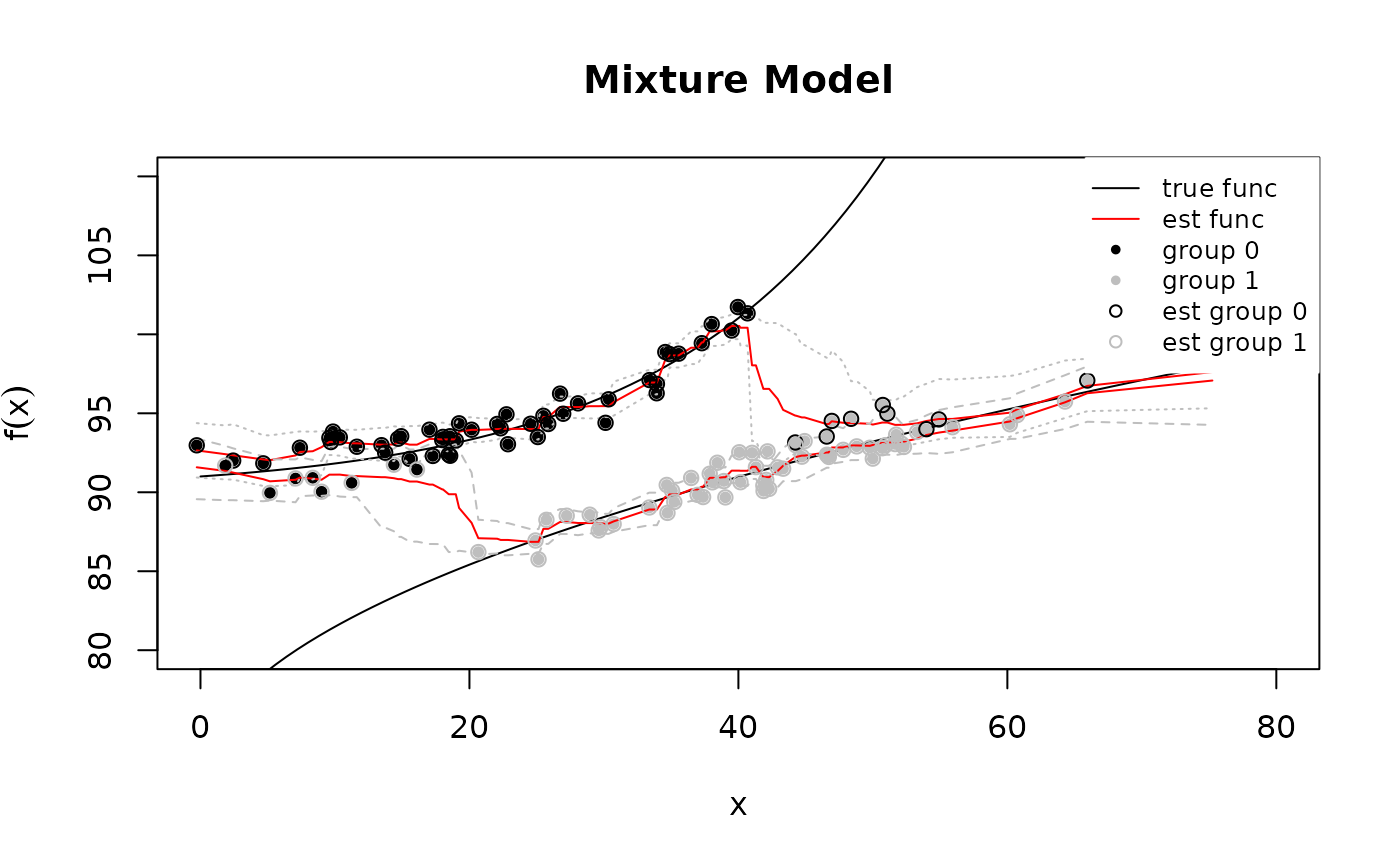
Several Forests with Multipliers
The sampler above holds one function. A model may want several, each entering the response through a multiplier the outer loop knows:
where are separate sums of trees and is a known per-observation scalar - an exposure, a dose, a treatment indicator, a group loading. Bayesian causal forests is the case with and .
One dbartsSampler per forest composes this in R, and the
composition is ordinary backfitting once the multiplier is folded in.
Given the residual
,
forest
’s
leaf conditionals want response
and precision weight
;
those are the two channels the loop writes, with setSigma
for the third and run(0L, 1L) to advance one sweep.
updateScale = FALSE (the default) is what makes the swap
coherent: every sweep’s residual is read on the scale creation fixed, so
the leaf prior keeps meaning what it meant.
A multiplier at or near zero says the row carries no information about that forest. Divide anyway and the response is amplified without bound, so the recipe snaps such a row to an exactly zero response paired with its exactly zero weight - which is what the engine does internally, at .
set.seed(919)
n.mf <- 200L
x.mf <- matrix(runif(n.mf * 3L), n.mf, 3L)
z.mf <- rbinom(n.mf, 1L, 0.5)
g1.true <- 2 * sin(pi * x.mf[, 1L])
g2.true <- 1 + 2 * x.mf[, 2L]
y.mf <- g1.true + z.mf * g2.true + rnorm(n.mf, 0, 0.5)

# the known per-observation multipliers, one vector per forest
m <- list(rep(1, n.mf), as.double(z.mf))
K <- length(m)

control.mf <- dbartsControl(n.chains = 1L, n.threads = 1L,
                            updateState = FALSE)
# every sampler is built on the SAME response, with k fixed and sigma owned
# by the outer loop
samplers <- lapply(seq_len(K), function(f)
    dbarts(x.mf, y.mf, control = control.mf, leaf.prior = normal(k = 1),
           family = gaussian(sigma = fixed(1)), n.trees = 25L))
# one prior budget divided among the forests, rather than K copies of the
# budget for the whole of the sum
base.mf <- samplers[[1L]]$getLeafPrior()$k.scale / samplers[[1L]]$getK()[1L]
for (s in samplers) s$setLeafPrior(normal(sd = base.mf / sqrt(K)))

g <- rep(list(rep(0, n.mf)), K)
sigma.mf <- 1
n.keep <- 200L
keep.g2 <- matrix(0, n.mf, n.keep)

for (i in seq_len(100L + n.keep)) {
  for (f in seq_len(K)) {
    r <- y.mf - Reduce(`+`, Map(`*`, m[-f], g[-f]))
    zero <- abs(m[[f]]) < sqrt(.Machine$double.eps)
    samplers[[f]]$setResponse(ifelse(zero, 0, r / ifelse(zero, 1, m[[f]])),
                              updateScale = FALSE)
    samplers[[f]]$setWeights(m[[f]]^2)
    samplers[[f]]$setSigma(sigma.mf)
    samplers[[f]]$run(0L, 1L)
    g[[f]] <- as.numeric(samplers[[f]]$getFitsWithoutOffset())
  }
  # sigma is drawn in R, against the COMBINED residual
  resid.mf <- y.mf - Reduce(`+`, Map(`*`, m, g))
  sigma.mf <- sqrt(sum(resid.mf^2) / rchisq(1L, n.mf))
  if (i > 100L) keep.g2[, i - 100L] <- g[[2L]]
}

c(recovery = cor(rowMeans(keep.g2), g2.true), sigma = sigma.mf, truth = 0.5)
## recovery sigma truth
## 0.9056196 0.4290352 0.5000000What it costs
Measured on one machine against a single batched engine sampler at matched total trees - the denominator matters, and a price quoted without one says nothing - K samplers driven a sweep at a time cost about 1.9-2.1 times that sampler at and 4.6-5.2 times at , growing roughly linearly in : each sampler pays its own per-sweep response install, weight install and result allocation over the full data. Driving one sampler a sweep at a time rather than in a batch is a separate and much smaller charge, about 1.1x.
Five things the recipe does not get
- No joint move on the multipliers. If the outer loop also draws the , it draws them in a block alternating with the forests. A sampler that holds both can interweave them instead, and the two mix differently whenever a forest and its multiplier are jointly weakly identified.
- The division is yours. The caller forms and so owns the conditioning, including the snap above.
- quantized predictor stores and sampler states, where one sampler holding forests keeps one of each.
- leaf calibrations to state, one per sampler, rather than a single calibration stated across the forests at creation.
- A serial outer loop. The forests are drawn one after another in R, so the composition cannot spread them across threads.
Graduating to a multi-forest sampler
dbarts(..., forests = list(forest(), forest(basis = factor(z))))
fits this model in one sampler, and the question a prototype should be
able to ask is whether moving to it changes the posterior being
targeted.
The additive decomposition ports exactly. What does not port by itself is prior shape. The two routes agree only if the caller
- centers
at its midrange, or absorbs the response transform’s shift with
setOffset: each single-forest sampler’s reported fit carries that shift, so the composition attributes it once per forest where the sampler attributes it once; - pins the leaf prior identically -
leaf.prior = normal(k)with fixed, every sampler built on a common , andupdateScale = FALSEthroughout; - accepts that with a multiplier far from 1 the internal response a forest sees leaves the band its leaf prior was calibrated for.
Without (1) and (2) the two routes are different priors that agree closely. With them the remaining difference is the leaf calibration alone. Measured on a pinned two-forest sampler against the recipe above, at over eight chains: with the remedies the posterior mean conditional effect agreed to 3.4% pointwise, inside Monte Carlo error in root-mean-square; without them the difference was 11.9% pointwise and several times Monte Carlo error. Both recovered the truth about equally well, which is the point - the difference is a prior, not a defect.
State equally plainly what the recipe does not reach and never will:
a response family, link or latent structure the sampler does not
provide, and a leaf or hyperprior it does not provide. Those are
selected by argument, not composed in R. forest() carries
the same scale knobs the composition sets by hand, and
$setForestBasis, $setForestWeights and
$getForestAmplitudes are the post-creation routes into a
multi-forest sampler, so a prototype ports without changing the model it
targets.
Response Families
Everything above fits a continuous response, dbarts’s
default (family = "auto", which chooses
"gaussian" for a continuous
and "probit" for one coded 0/1). family can
also be set to "gaussian", "probit", or
"logistic" explicitly. The two binary families model
for a link
and the sum-of-trees
,
and report fits and predictions on that latent scale rather than as
probabilities (pnorm/plogis recovers the
probability from it). Probit takes
to be the standard normal CDF; logistic uses Polya-Gamma augmentation
and takes
to be the logistic CDF, whose latent variable has heavier tails than
probit’s, so the leaf-value prior widens to match (its scale becomes pi
* sqrt(3) in place of probit’s 3), without naming the slot.
DART
When only a handful of predictors out of many are relevant, the CGM
tree prior’s uniform choice of split variable wastes proposals on the
rest. split.probs = dart(...) replaces it with a Dirichlet
prior over split-variable probabilities (Linero 2018): the sampler
learns which variables matter and increasingly proposes splits on them,
which doubles as a variable-importance diagnostic.
set.seed(12)
n.dart <- 60
x.dart <- matrix(runif(n.dart * 8), n.dart)
y.dart <- 4 * x.dart[, 1] + rnorm(n.dart, 0, 0.2)

fit.dart <- dbarts(y.dart ~ x.dart, split.probs = dart(),
                   control = dbartsControl(n.burn = 100L,
                                            n.chains = 1L, n.threads = 1L),
                                            n.trees = 10L)
samples.dart <- fit.dart$run(100L, 30L)

# One row per predictor, averaged over the retained samples: only the first
# column of x.dart drives y.dart, and its split probability dominates.
round(rowMeans(samples.dart$varprobs), 3)
## [1] 0.991 0.000 0.005 0.001 0.000 0.000 0.001 0.002The Dirichlet concentration alpha is itself sampled by
default (update.alpha = TRUE); a smaller alpha
concentrates the split probabilities more aggressively.
?dbartsPriors documents the rest of dart’s
arguments.
Data Frames, Factors, and Missing Values
dbarts and bart take a
data.frame directly, and
(factors = "categorical", the default for both) an
unordered factor predictor becomes a single categorical column: its
splits send a subset of levels down each branch, rather than the
one-indicator-per-level expansion bartBT still uses.
factors = "indicators" recovers that expansion on either
function, useful for comparing the two. Ordered factors are their own
predictor kind regardless of factors: coded on their
integer levels and split at a threshold, with one candidate threshold
per level boundary rather than a fixed count of cuts, so
n.cuts does not reach them.
Missing predictor values need not be removed beforehand. By default
every split rule learns a direction for NA: an observation
whose split variable is missing follows that rule’s direction (“Missing
Incorporated in Attributes”, Twala et al. 2008), estimated jointly with
the rest of the tree. na.action = na.fail instead refuses
any missing value, the response’s too.
set.seed(13)
n.miss <- 60
g <- factor(sample(c("a", "b", "c"), n.miss, replace = TRUE))
x.miss <- rnorm(n.miss)
x.miss[sample(n.miss, 10)] <- NA
y.miss <- ifelse(g == "a", 2, -1) +
    ifelse(is.na(x.miss), 0, x.miss) + rnorm(n.miss, 0, 0.2)

df.miss <- data.frame(y = y.miss, x = x.miss, g = g)
fit.miss <- bart(y ~ x + g, df.miss, n.trees = 10L, n.chains = 1L,
                  n.threads = 1L, n.samples = 20L, n.burn = 20L,
                  verbose = FALSE)
g above ingests as one categorical predictor with three
levels rather than two indicator columns, and the ten missing values of
x are incorporated rather than dropped.
A Random-Intercept Model Through setOffset
The response-side conduit carries a whole outer block just as
setPredictor carries the predictor side. A random-intercept
model
is the smallest worked example:
and
are two Gibbs blocks the outer loop owns, and BART sees them only as an
offset. Each sweep draws
from its conjugate normal against the current residual, installs
’s
new offset with setOffset, runs one sweep, subtracts the
offset back off the reported fit, and then draws
.
setOffset(offset, updateScale) takes
updateScale = FALSE after warmup: the response transform
BART calibrated at creation must stay put, or
and
- which the outer loop holds in response units - would come to mean
something else from one sweep to the next.
set.seed(24)
n_ri     <- 200L
n_groups <- 8L
g        <- rep_len(seq_len(n_groups), n_ri)
x_ri     <- matrix(runif(n_ri * 3L), n_ri, 3L)
b_true   <- rnorm(n_groups, 0, 0.8)
y_ri     <- sin(pi * x_ri[, 1L]) + 2 * x_ri[, 2L] + b_true[g] + rnorm(n_ri, 0, 0.5)

n_warmup_ri  <- 200L
n_samples_ri <- 500L

control_ri <- dbartsControl(updateState = FALSE, verbose = FALSE,
                            n.burn = 0L, n.samples = 1L, n.chains = 1L,
                            n.threads = 1L)
sampler_ri <- dbarts(x_ri, y_ri, control = control_ri, n.trees = 50L)

# rows of each group, and its size; the conjugate draw needs both
rows_of  <- split(seq_len(n_ri), g)
size_of  <- lengths(rows_of)

# Half-Cauchy(0, 2.5 sd(y)) on tau, sampled by a random-walk Metropolis step
tau_scale <- 2.5 * sd(y_ri)
log_tau_posterior <- function(tau, b) {
  if (tau <= 0) return(-Inf)
  -n_groups * log(tau) - 0.5 * sum(b^2) / tau^2 +
    dcauchy(tau, 0, tau_scale, log = TRUE)
}

b     <- rnorm(n_groups, 0, tau_scale / 5)
tau   <- tau_scale / 5
sigma <- sd(y_ri)
f_hat <- rep_len(0, n_ri)

samples_b   <- matrix(NA_real_, n_samples_ri, n_groups)
samples_tau <- rep_len(NA_real_, n_samples_ri)

for (i in seq_len(n_warmup_ri + n_samples_ri)) {
  # b | f, sigma, tau: independent normals, one per group
  resid     <- y_ri - f_hat
  post_var  <- 1 / (size_of / sigma^2 + 1 / tau^2)
  post_mean <- post_var * (vapply(rows_of, function(rows) sum(resid[rows]), 0) /
                             sigma^2)
  b <- rnorm(n_groups, post_mean, sqrt(post_var))

  # f, sigma | b: one BART sweep against the intercepts as an offset. The
  # scale re-anchors during warmup only, and is pinned for every kept draw.
  sampler_ri$setOffset(b[g], updateScale = i <= n_warmup_ri)
  draw  <- sampler_ri$run()
  f_hat <- as.vector(draw$train) - b[g]
  sigma <- draw$sigma[1L]

  # tau | b: a random-walk Metropolis step on the log scale
  proposal <- tau * exp(rnorm(1, 0, 0.2))
  logRatio <- log_tau_posterior(proposal, b) - log_tau_posterior(tau, b) +
    log(proposal) - log(tau)
  if (log(runif(1)) < logRatio) tau <- proposal

  if (i > n_warmup_ri) {
    samples_b[i - n_warmup_ri, ] <- b
    samples_tau[i - n_warmup_ri] <- tau
  }
}

# the group intercepts and their scale are only identified up to a shared
# level, which the forest absorbs, so compare them centered
cor(colMeans(samples_b) - mean(colMeans(samples_b)), b_true - mean(b_true))
## [1] 0.99589The same shape carries any outer block whose contribution to the
linear predictor is a per-observation vector: a parametric term, a
spatial effect, a frailty. setResponse is the companion for
a block that changes
itself rather than shifting it.
Multiple Threading
When implementing a Gibbs sampler using dbarts in R, it
is most often the case that multiple threads will need to be handled by
creating separate copies of the sampler and data. While
dbartsSamplers are natively multithreaded, few of their
slots are stored independently across chains, so an outer loop that owns
per-chain state runs one single-chain sampler per chain and threads them
itself.
This custom-loop bookkeeping is only needed when embedding BART in a
larger sampler. A plain multi-chain bart fit already tracks
its chain dimension: summary() reports split-R-hat and
effective sample size for the scalar parameters the fit sampled
(sigma, and k when it is drawn) and names any
it held fixed on a line under the table, and
dbarts::extract(fit, "sigma", combineChains = FALSE)
returns a sampled parameter’s draws chain-separated, as a
chains-by-samples matrix; a parameter held fixed comes back as its one
number.