Bayesian Additive Regression Trees
bartBT.RdBART is a Bayesian “sum-of-trees” model in which each tree is constrained by a prior to be a weak learner.
For numeric response \(y = f(x) + \epsilon\), where \(\epsilon \sim N(0, \sigma^2)\).
For binary response \(y\), \(P(Y = 1 \mid x) = \Phi(f(x))\), where \(\Phi\) denotes the standard normal cdf (probit link).
bartBTis the BayesTree-compatible surface: 0.9-34's argument list exactly, no new features, and nofamilyargument at all - every fit is the default gaussian/probit pair above.bartreaches every other response family - logistic, accelerated failure time, discrete-time survival hazard, K-category multinomial, ordered categorical, negative-binomial counts, and semicontinuous two-part responses - plus its own formula-term multi-forest interface.
Usage
bartBT(
    x.train, y.train, x.test = matrix(0.0, 0, 0),
    sigest = NA, sigdf = 3, sigquant = 0.90,
    k = 2.0,
    power = 2.0, base = 0.95, splitprobs = 1 / numvars,
    binaryOffset = 0.0, weights = NULL,
    ntree = 200,
    ndpost = 1000, nskip = 100,
    printevery = 100, keepevery = 1, keeptrainfits = TRUE,
    usequants = FALSE, numcut = 100, printcutoffs = 0,
    verbose = TRUE, nchain = 1, nthread = 1, combinechains = TRUE,
    keeptrees = FALSE, keepcall = TRUE, sampleronly = FALSE,
    seed = NULL,
    proposalprobs = NULL,
    keepsampler = keeptrees)

# S3 method for class 'bart'
plot(
    x,
    plquants = c(0.05, 0.95), cols = c('blue', 'black'),
    ...)

# S3 method for class 'bart'
predict(
    object, newdata,
    type = c("ev", "ppd", "bart", "forest", "sigma"),
    offset = NULL, weights = NULL,
    combineChains = TRUE,
    ci.level = NULL,
    forest = NULL,
    bases = NULL,
    na.action = dbarts::na.keepPredictors,
    n.threads,
    ...)

# S3 method for class 'bart'
print(x, ...)

extract(object, ...)
# S3 method for class 'bart'
extract(
    object,
    type = c("ev", "ppd", "bart", "loglik", "trees", "forest",
             "sigma", "k", "leaf.prior.sd", "varcount"),
    sample = c("train", "test"),
    combineChains = TRUE,
    forest = NULL,
    contribution = FALSE, ...)

# S3 method for class 'bart'
fitted(
    object,
    type = c("ev", "ppd", "bart", "forest"),
    sample = c("train", "test"),
    ci.level = NULL,
    ...)

# S3 method for class 'bart'
residuals(object, type = "ev", ...)

# S3 method for class 'bart'
family(object, ...)
Arguments
- x.train
Explanatory variables for training (in sample) data. May be a matrix or a data frame, with rows corresponding to observations and columns to variables. If a variable is a factor in a data frame, it is replaced with dummies. Note that \(q\) dummies are created if \(q > 2\) and one dummy is created if \(q = 2\), where \(q\) is the number of levels of the factor. A sparse
Matrix::dgCMatrixof ordinal predictors is also accepted, as is a data frame mixing ordinary columns withMatrix::sparseVectorordgCMatrixcolumns; seedbarts.- y.train
Dependent variable for training (in sample) data. If
y.trainis numeric a continuous response model is fit (normal errors). Ify.trainis a two-level factor (or logical, or two-level character) or has only values 0 and 1, then a binary response model with a probit link is fit. A factor with three or more levels is an error, whose message names both remedies:bart(x, y, family = "multinomial")for a multinomial fit, oras.integer(y) - 1Lto keep the numbers dbarts 0.9-x fit from the level codes.- x.test
Explanatory variables for test (out of sample) data. Should have same column structure as
x.train.bartBTwill generate draws of \(f(x)\) for each \(x\) which is a row ofx.test.- sigest
For continuous response models, an estimate of the residual standard deviation (residual standard error), \(\sigma\), used to calibrate an inverse-chi-squared prior on the error variance. A positive number, or one of
"auto","dense"and"sparse", naming how one is made: each gives the residual standard deviation of the linear regression of the response on the predictors, factors entering as indicator columns whatever the trees are given, and, where that regression leaves no residual degrees of freedom, the standard deviation of the response over the observations of positive weight, weighted as the regression is (summary(lm(y ~ 1, weights = weights))$sigma,sd(y)at unit weights), which a line underverboseand one in the fit'ssummarysay, with no warning. (Where rows are out and the observations of positive weight hold fewer than two distinct values of the response, the regression is made on every row instead, under the warning of classdbartsScaleFallbackWarning.)"auto"islm's own routine ("dense") for a matrix or a data frame and an exact sparse one ("sparse") where the caller supplied a sparse-stored column.NA(the default) is"auto"; the lines underverboseare printed with the rest of this function's output.dbartssays what the two routines cost, where they differ, and what to pass in place of an expensive estimate, which cannot be interrupted once begun. Seesigquantfor more information. Not applicable when \(y\) is binary. Same concept assigestindbartsandxbart.- sigdf
Degrees of freedom for error variance prior. Not applicable when \(y\) is binary. Default 3, Chipman, George, and McCulloch's calibration (see References); an aggressive choice rather than a derived one.
- sigquant
The quantile of the error variance prior that the rough estimate (
sigest) is placed at. The closer the quantile is to 1, the more aggressive the fit will be as you are putting more prior weight on error standard deviations (\(\sigma\)) less than the rough estimate. Not applicable when \(y\) is binary. Default 0.90, from the same source assigdf.- k
For numeric \(y\),
kis the number of prior standard deviations \(E(Y|x) = f(x)\) is away from \(\pm 0.5\). The response (y.train) is internally scaled to range from \(-0.5\) to \(0.5\). For binary \(y\) fit with the default probit link,kis the number of prior standard deviations \(f(x)\) is away from \(\pm 3\), the probit reference scale;family = "logistic"widens this to \(\pm \pi \sqrt{3}\), which is three standard deviations of the standard logistic latent variable (\(\pi / \sqrt{3}\) each), the same three-sd span probit's \(\pm 3\) covers. In both cases, the bigger \(k\) is, the more conservative the fitting will be. The value can be either a fixed number, or a hyperprior of the formchi(df = 1.5, scale = 2).bartBT's own default is the fixed value 2; seebart'skitem for itsNULLdefault, achi(1.5, 2)hyperprior on binary responses. The default of 2 for continuous responses follows Chipman, George, and McCulloch's argument (see References) that with leaf prior standard deviation \(\sigma_\mu = 0.5 / (k \sqrt{m})\) for \(m\) trees, \(k\) prior standard deviations of \(f(x)\) span the whole coded response range regardless of \(m\) – so \(k = 2\) places that range at roughly a 95% prior interval. The range scaling itself is an outlier-sensitive convention shared with BayesTree/bartMachine: extreme \(y\) values compress the effective prior on everything else, for which the published workaround is to log-transform or winsorize such values before fitting, or to letkadapt via thechihyperprior. A writtenNULLis refused, saying to leave the argument out for its default.- power
Power parameter for tree prior. Default 2, Chipman, George, and McCulloch's empirical recommendation (see References) for the split-probability decay \(base (1 + depth)^{-power}\), not derived from a formula. A written
NULLis refused, saying to leave the argument out for its default.- base
Base parameter for tree prior. Default 0.95, from the same source as
power. A writtenNULLis refused, saying to leave the argument out for its default.- splitprobs
Prior and transition probabilities of variables used to generate splits. Can be missing/empty/
NULLfor equiprobability, a numeric vector of length equal to the number variables, or a named numeric vector with only a subset of the variables specified and a.defaultnamed value. Values given for factor variables are replicated for each resulting column in the generated model matrix. The symbolnumvarsis rebound before execution to the number of columns in the model matrix.- binaryOffset
Used for binary \(y\). When present, the model is \(P(Y = 1 \mid x) = \Phi(f(x) + \mathrm{binaryOffset})\), allowing fits with probabilities shrunk towards values other than \(0.5\). \(\Phi\) is the link for the default probit family; a
family = "logistic"fit usesplogisinstead, as noted in the value section below.- weights
An optional vector of weights to be used in the fitting process. For a gaussian response, BART fits a model with observations \(y \mid x \sim N(f(x), \sigma^2 / w)\), where \(f(x)\) is the unknown function. A probit fit (
bartBT, orbartwith the default binary family) does not support weights, except that weights identically 1 are treated as absent, and weights that are all 0 and 1 name the rows in the data set, a 0 row leaving the likelihood but keeping its leaf occupancy, its latent and its fitted value (the same holds forfamily = "ordinal"); afamily = "logistic"fit treats them as observation counts and requires non-negative whole numbers no larger than \(10^6\), as a sweep's time grows with the total count, a count of 0 leaving the row out of the likelihood. A training row's"ppd"draw is one observation like the row, one 0/1 draw on a binary fit whatever its weight;predict'sweightson a binary fit are trial counts, drawing \(\mathrm{Binomial}(w, p)\) successes with \(p\) the fitted probability, a 0 drawing none (seebart'sweightsitem). A row at weight 0 hasNA"ppd"draws on every family and in every route: a training row (extract,fitted(type = "ppd")), a row of the test sample whose test-frame weight is 0, and, on a gaussian or Student-t fit, a row givenweightsof 0 topredict; anaftfit takes no case weights at fit time, so onlypredict(weights = )reaches a weight of 0 on it, with the same result. A weight of 0 holds a row out of the fit, and on a gaussian fit gives it no noise scale, \(\sigma / \sqrt{w}\), assimulategivesNaNat a weight-0 row of anlmfit; no warning is raised, and every other row's draw is as it would be without the row. To draw such a row as a new observation, state its weight:predict(fit, type = "ppd", weights = 1).- ntree
The number of trees in the sum-of-trees formulation. A data object holding the bases of a sampler of several forests fits one forest here, as
dbartsdoes given noforests. Like every count on this page (nskip,ndpost,numcut,keepevery,printevery,nthread,nchain,printcutoffs), a fractional value is refused, naming the argument, rather than silently truncated; seedbartsControlfor the shared whole-number rule. A writtenNULLis refused, saying to leave the argument out for its default.- ndpost
The number of posterior draws after burn in,
ndpost / keepeverywill actually be returned.- nskip
Number of MCMC iterations to be treated as burn in.
- printevery
As the MCMC runs, a message is printed every
printeverydraws.- keepevery
Every
keepeverydraw is kept to be returned to the user. Useful for “thinning” samples.- keeptrainfits
If
TRUEthe draws of \(f(x)\) for \(x\) corresponding to the rows ofx.trainare returned.- usequants
When
TRUE, determine tree decision rules using estimated quantiles derived from thex.trainvariables. WhenFALSE, splits are determined using values equally spaced across the range of a variable, or, for a variable with fewer distinct values thannumcut, half-way between neighboring values. See details for more information.- numcut
The maximum number of possible values used in decision rules (see
usequants, details). A single number applies to every column; otherwise a vector of length equal toncol(x.train), or named asbart'sn.cutsreads. Fewer rules may be used if a covariate lacks enough unique values.- printcutoffs
The number of cutoff rules to printed to screen before the MCMC is run. Given a single integer, the same value will be used for all variables. If 0, nothing is printed.
- verbose
Logical; if
FALSEsuppress printing.- nchain
Integer specifying how many independent tree sets and fits should be calculated. Default 1 for
bartBT, BayesTree's historical single-chain convention;bart's default is 4.- nthread, n.threads
A positive integer giving a total thread budget, distinct from
nchain: chains run in parallel across it, but tree sampling itself uses at most one thread per chain, so a budget abovenchainbuys the sampler's own sweep nothing. The surplus still feeds the test-fit pool andpredict's own fan-out, and a fit warns once, naming both counts, when an explicit budget exceeds the chain count.bartBT's default is 1.On
predict,n.threadsis a per-call worker count for the saved-tree replay, defaulting to the fit's own: the replay is partitioned by (chain, posterior draw), each partition writing its own rows and nothing being reduced across workers, so the answer is identical bit for bit at every value and only the time taken changes. It is the last positional argument of everypredictmethod, so a caller that passes arguments by position is unaffected by its presence. A value that is not a single positive number is an error rather than a silent fallback.- combinechains, combineChains
Logical; if
TRUE, samples from every chain are collapsed into a single matrix/vector ofnchain\(\times\)ndpostrows (see ‘Value’ for the row order); ifFALSE, they are kept in arrays of dimensions equal tonchain\(\times\)ndpost\(\times\) number of observations. DefaultTRUEacrossbartBTandbart; the number of chains is tracked regardless on the returned object'sn.chainscomponent (see ‘Value’). Onextract,predictandsurvivalProbabilities,FALSEkeeps that leadingnchainmargin - length 1 on a one-chain fit - rather than dropping it there; a scalar type (sigma,k, a component'sshape) is then a 1 x samples matrix instead of a plain vector. A fit's own STOREDcombinechains = FALSEfields keep 0.9-x's one-chain collapse instead, so$yhat.trainand its siblings never gain that margin on their own.- keeptrees
Logical; must be
TRUEin order to usepredictwith the result of abartfit. Note that for models with a large number of observations or a large number of trees, keeping the trees can be very memory intensive. The methods read the kept sampler asbart'skeepTreesitem describes; running it further is not a supported use of the fit.- keepcall
Logical; if
FALSE, returned object will havecallset toNULL, otherwise the call used to instantiate BART.- seed
Optional integer specifying the desired pRNG seed.
NULL(the default) leaves the fit unseeded, and an explicitNAis a missing value, as inset.seed: it reads asNULLfor one release, with a once-per-session warning; aset.seedbeforehand then suffices for reproducibility. Supplyingseedinstead gives reproducible results without touching R's stream. See the Reproducibility section of bart.- proposalprobs
Named numeric vector or
NULL, optionally specifying the proposal rules and their probabilities. Elements should be"birth_death","swap","change","perturb"and"rule_gibbs"to control tree structure proposals, and"birth"to give the relative frequency of birth/death in the"birth_death"step.NULL(the default), or a vector naming none of"birth_death","swap"and"change", takes BayesTree's mixture for those three,c(birth_death = 0.5, swap = 0.1, change = 0.4), as 0.9-x did (birthdefaults to 0.5 either way); any other vector is completed asdbartsControlcompletes one.bart's default differs:c(birth_death = 0.6, swap = 0, change = 0.4, perturb = 0, rule_gibbs = 0, birth = 0.5). All five structural probabilities zero is the frozen mixture: no structural proposal is made, the tree structures stand where they are, and only the leaf values,sigmaand the family's latents keep being drawn, which is how a fitted forest is re-sampled as a fixed basis. UnderdbartsControl's defaulttreeShift = "auto"a frozen forest additionally takes the level-shifting Gibbs step each iteration, the leaf values then being the only thing left to move.bartBThas notreeShiftformal of its own and always runs at this default;bartand adbartssampler's control object can set it to"always"or"never"instead, which changes the sampled values without changing the posterior. A"swap"element exchanges a parent's split rule with a child's;bartships it at zero because at forests of 75 trees and more dropping it changed accuracy, coverage and mixing little in simulation (see NEWS), andbartBTkeeps it at 0.1 to match BayesTree. Withn.trees = 1it is the only move that rotates a rule up the tree. A"perturb"element displaces one node's split point by a single cut position while keeping its variable and the tree's shape; it defaults to zero, and only ordinal (numeric) columns can be perturbed. A"rule_gibbs"element replaces one nog node's rule - a node whose two children are both leaves - with a draw from that rule's own full conditional over the available ordinal variables and their admissible cuts, so its acceptance is one; it defaults to zero, it acts only where the node's own rule is ordinal, and it is inert on an all-categorical design.- keepsampler
Logical that can be used to save the underlying
dbartsSampler-classobject even ifkeeptreesis false.- object
An object of class
bart, returned from either the functionbartBTorbart.- newdata
Test data for prediction. Obeys all the same rules as
x.train, except that on a fit with a factor column a numeric matrix is refused by name, and a data frame is given. An unnamed matrix is read in the fit's column order, with no message. Left out (orNULL),predictreturns eachtypeat the training rows from the draws the fit stored, asextractwithsample = "train"does, and needs no saved trees; anoffsetgiven then replaces the fit's own at the training rows, one value or one per training row;weightsreplace the fit's own weights for the training rows'"ppd"draws, one value or one per training row, acting as they do atnewdatafor each family (seetype); andbasesreplace the fit's own bases there (seebases). The offset and the weights are checked against the number of training rows, one value or one per row, and weights, here and atnewdata, are a vector or a one-column matrix, a matrix of several columns, a data frame or a list being refused. A missing value in a per-row offset or weights is answered byna.actionexactly as atnewdata: the default andna.failrefuse it,na.passreturns that row withNAdraws,na.omitdrops the row from the result andna.excludepads it back asNA; a single missing value is always refused. The weights' values are looked at, as atnewdata, by a"ppd"draw alone, which refuses those its family cannot take, and any other type takes whatever they hold. The bases are checked as atnewdata. None needs saved trees, and a fit kept without its training draws is refused by name.- offset
For
predict: an optional offset fornewdata, applied the same waydbarts'soffset.testis at fit time. It shifts the PREDICTED rows, not the training ones - a different channel fromoffset.test, which is why it carries its own name rather than that one's.NULL(the default, when missing) takes the fit's own offset: itsbinaryOffset, and theoffset()terms andoffsetargument of a formula fit evaluated onnewdata, a plain vector for the training rows applying only to anewdataof as many rows. A givenoffsetis added to abinaryOffset. Refused, by name, withtype = "forest": an offset shifts the recombination of the forests, never any one forest's own total, so it belongs to the arithmetic under ‘Value’ rather than to what comes back. On an amplitude-coupled fit's combined arms (type = "ev","ppd","bart") it is that recombination, and enters the sum of trees before the family's link, exactly as it does for a single forest.- sampleronly
Builds the sampler from its arguments and returns it without running it. Useful to use the
bartBTinterface in more complicated models.- x
Object of class
bart, returned by functionbartBT, which contains the information to be plotted.- plquants
In the plots, beliefs about \(f(x)\) are indicated by plotting the posterior median and a lower and upper quantile.
plquantsis a double vector of length two giving the lower and upper quantiles.- cols
Vector of two colors. First color is used to plot the median of \(f(x)\) and the second color is used to plot the lower and upper quantiles.
- type
The quantity to be returned by generic functions. Options are
"ev"- samples from the posterior of the individual level expected value,"bart"- the sum of trees component; same as"ev"for linear models but on the latent scale (probit or logistic, matching the fit's family) for binary ones,"ppd"- samples from the posterior predictive distribution,"loglik"- forextractonly, the log-likelihood of each training observation at each posterior draw (a row whose weight is a count has its value multiplied by the count; a row with a precision weight of zero, or masked out of the data, is not in the likelihood and isNaN, so drop those columns before handing the matrix to a tool such as loo),"trees"- a data frame with tree information for when model was fit withkeepTreesequal toTRUE, and"forest"- forextract,predictandfitted, the per-forest channels of an amplitude-coupled multi-forest fit (seeforest,contribution, and theforestFits/glue/basescomponents under ‘Value’); an error naming the reason on any other fit, abartmultinomial one included, whose K forests are per-category latents rather than additive components of one location.extract(type = "forest")reads the stored in-sample channel, whilepredict(type = "forest")replays each forest atnewdata; both report the raw per-forest total, leaving the recombination to the caller, where the combined arms ("ev","ppd","bart") perform it given the bases at those rows (seebases).fitted(type = "forest")is the posterior mean of whatextractreports, a rows-by-forests matrix withextract's dimnames, pooled over all samples and chains and refused whereverextractrefuses it; it is each forest's own total BEFORE its basis and amplitude multiply it, so it is not that forest's contribution to the fitted value, andresidualsrefuses it. For"ppd", a weighted logistic fit draws the number of successes among the observation-count weight, \(\mathrm{Binomial}(w_i, p_i)\) (seeweights), andweightsgiven topredicton a probit or logistic fit are likewise trial counts, positive integers, each new row drawing \(\mathrm{Binomial}(w_i, p_i)\), an aft (survival) fit draws on the log-time scale (the fit models \(\log T\)), afamily = student()fit draws \(f + \sigma t_\nu / \sqrt{w_i}\) at each draw's own \(\sigma\) and \(\nu\) (the fit's$resid.df), and a heteroscedastic fit (dbarts'svariance) draws its noise at that observation's own \(s(x_i)/\sqrt{w_i}\). For"loglik", gaussian fits evaluate \(y_i \mid x_i \sim N(\hat{f}(x_i), \sigma^2 / w_i)\) in logs at each draw of \(f\) and \(\sigma\) - or, for a heteroscedastic fit, \(y_i \mid x_i \sim N(\hat{f}(x_i), s^2(x_i) / w_i)\) at each draw of \(f\) and \(s\), afamily = student()fit the corresponding marginal \(t_\nu\) density at that draw's \(\nu\) (the fit's$resid.df) rather than the normal one, binary fits evaluate the Bernoulli log-likelihood of the fitted probability, multiplied for a weighted logistic fit by the observation-count weight \(w_i\), and an aft fit contributes the log density for an event and the log survival tail \(\log P(T > C)\) for a right-censored observation, both on the log-time scale: an event's term is the density of \(\log T\), which exceeds the density of \(T\) by \(\log t\), so to compare with a model of \(T\), subtract \(\log t\) at each event. When chains are combined the result is a samples-by-observations matrix directly consumable by WAIC/PSIS-LOO implementations such as those in the loo package; the chains-first convention is kept, so a per-chain array (combineChains = FALSE, dimension chains-by-samples-by-observations) is reordered to the draws-by-chains-by-observations thatloo::relative_effexpects withaperm(x, c(2, 1, 3)). To synergize withpredict.glm,"response"can be used as a synonym for"ev"and"link"can be used as a synonym for"bart"; thebartextended-family methods take the same two synonyms, each against its own set of types.extractalso takes"sigma","k"and"leaf.prior.sd", the residual scale, the leaf prior'skand its standard deviation, and"varcount", the per-predictor split counts shaped as"ev"is with predictors in place of observations - none of them per-observation, so a suppliedsampleis refused by name on all of them. A parameter the fit sampled comes back as its draws, a chain-combined vector or (combineChains = FALSE) a chains-by-samples matrix; one the fit held fixed comes back as that one number, under eithercombineChains, andforestselects among the forests of a fit with several (seeforestbelow and the ‘Leaf prior parameterk’ subsection).sigmaon a weighted fit is the scale at weight 1 (row i's is \(\sigma / \sqrt{w_i}\)); on afamily = student()fit it is the t scale, not the standard deviation. A fit whose family has no residual scale to estimate - probit, logistic, hazard, and the ordinal, negative-binomial and multinomial fits ofbart- answers"sigma"with 1, assigmadoes on a binomialglm. A heteroscedastic fit's"sigma"is its per-observation scale \(s(x)\), laid out as"ev"is and takingsample:extractreturns the storeds.trainors.test, andpredict, which takes"sigma"on such a fit only, evaluates the variance forest atnewdata(refusingweights, since a case weight does not change \(s(x)\)). For information on extracting trees, see the subsection below.- sample
Either
"train"or"test"."test"is refused, by name, whentypeis"forest": an amplitude-coupled fit has no test fits (seedbarts'sforests =). It isextract's andfitted's own argument -fittedis always the training rows - and is refused by name onpredict, whose stored train and test channels areextract'ssampleinstead; also refused by name onextract(type = "sigma")/"k"/"leaf.prior.sd"/"varcount", none of them per-observation ("sigma"excepted on a heteroscedastic fit, where it is).- forest
For
extract(type = "forest"),extract(type = "trees")andpredict(type = "forest"): which forest(s) to return, by 1-based position, as base R reads a list element by number, or by label (a string; seeforest),"forest1","forest2", ... naming position i when a forest is selected (the margins themselves are named by the forests' labels, asforest<i>for a forest with none);NULL(the default) returns every forest. Fortype = "forest"the returned array always keeps the trailing forest margin, subset to the requested forests, even when only one is selected;type = "trees"returns a data frame and keeps no such margin. Forextract(type = "k")andextract(type = "leaf.prior.sd")on a fit with several forests, it selects among the per-forest entries, which both name by the forests' labels (the entry itself for a single forest). Selecting a forest outside those is refused by name: every other arm has already recombined the forests into the location it reports, except"sigma"(a model parameter with no forest axis) and"varcount"(which already keeps every forest on its own trailing margin), each naming its own reason instead.- bases
For
predicton an amplitude-coupled multi-forest fit: the bases each forest's amplitudes multiply AT the predicted rows, which off the training rows only the caller knows. A list with one entry per forest, in the forests' order, or with entries named by the forests' labels (forest<i>also selects position i), entry k eitherNULL(for a forest that declared no basis, whose amplitude multiplies an implicit all-ones column) or a value of the class the forest was created with, which decides what it multiplies (seeforest'sbasisitem) and cannot change. A single string names a column ofnewdata,bases = "dose"readingnewdata$dose, on any number of rows, one included; a level is given as a factor,factor("trt", levels = c("ctl", "trt"))on one row. For a forest of levels, created with a factor, a character vector or a logical vector, hand over a factor, a character vector or a logical vector: its levels are matched to the forest's by name and not by position, a level of the forest that no row has is a column of zeros, and a row at a level the forest does not have, or atNA, is refused. Numbers are refused for such a forest, a factor's indicator columns among them: hand over the factor itself,fit$basesholding it. For a forest of numbers, hand over its one numeric column, a vector or a matrix of one column; several columns, a factor, a character vector and a logical vector are refused (as.numeric()of a logical vector is its 0/1 column). Either way it is required to havenrow(newdata)rows, or as many rows as the fit has training rows whennewdatais left out; with nonewdata,basesreplace the fit's own at the training rows, which is the counterfactual at the rows the fit was made on. The fit is then rebuilt draw by draw from the per-forest channels it stores (forestFits,glueandbases; see ‘Value’), with no saved trees, everytypereading off the rebuilt total, and anoffsetgiven with them applies as well; a fit kept without those channels (keepFits = FALSE) is refused, saying to refit withkeepFits = TRUE. A missing value is refused on a row the prediction keeps and passed by on a row thena.actiondrops (seena.keepPredictors). A named entry selects the forest whose label it is and an unnamed one the forest at its position, in any order and any subset; a forest no entry names is left as it is, which atnewdatais an error for a forest that carries a basis, and two entries for one forest are refused. When exactly one forest carries a basis the bare value may be given on its own, without the list: for a Bayesian causal forest fit with its arm asfactor(z),bases = factor(zstar, levels = levels(factor(z)))is the counterfactual arm being predicted under, andbases = fit$basesat the training rows is the training fit, to rounding. With nonewdataaNULLentry for a forest that carries a basis is refused, as atnewdata, since it does not stand for the fit's own; the message names the way to keep the fit's own bases and change others,b <- fit$bases; b[[2]] <- z1; predict(fit, bases = b). Unlike at fit time, a column of all zeros on a forest of numbers and, on a forest of levels, a factor or a character vector with every row at one of the forest's levels are accepted, since a constant arm is the point of a counterfactual.NULL(the default) builds each basis again fromnewdatawhen the fit's forest wrote it as code, in abartordbartsformula'sforest()term or in aforestslist (it then needs the columns of the fit's data that basis names, coded against the fit's own factor levels; seeforest'sbasisitem), and is an error naming the forest when the basis was handed over as a value or needs a variable that had a value for every fitted row and is no column ofnewdata. Refused on a single-forest fit, and withtype = "forest", which reports each forest's total before any basis.- contribution
For
extract(type = "forest")only:FALSE(the default) returns the raw per-forest totalforestFitsalready carries (see ‘Value’).TRUEinstead returns each selected forest's per-observation CONTRIBUTION to the fit, \((\mathrm{basis}_k \, \mathrm{glue}_k) \times \mathrm{forestFits}_k\), computed on demand from the storedforestFits,glue, andbasesrather than stored itself.- na.action
For
predict: what to do with the rows ofnewdatathat have missing values, and, with nonewdata, the training rows whose per-rowoffsetorweightshas one; see ‘At Prediction’ inna.keepPredictors.- ci.level
For
fittedandpredict, an optional single number in \((0, 1)\). WhenNULL(the default), each generic returns what it always has:fittedthe posterior mean,predictthe full array of posterior samples (seetypeabove), unsummarized. When given, the result is instead a matrix with one row per observation and columnsest(the posterior mean),ci.lower, andci.uppergiving a symmetric credible band at that level, pooled over all samples and chains. The kind of interval followstype:"ev"yields a credible interval for the conditional mean (a probability for binary responses),"ppd"a prediction interval that additionally carries the residual noise (and so is wider), and"bart"a credible interval on the latent scale. A row with no draws, a weight-0 row of a posterior predictive draw (seeweights), hasNAin all three columns. Forfitted(type = "forest")it returns the rows-by-forests-by-3 array ofest,ci.lowerandci.upper, as for a multinomial fit;predict(type = "forest")refuses it by name, since that arm reports each forest's own total before any basis. It is also refused onresiduals, where it would band a constant minus an increasing triple and so mislabel two of its three columns; takey - fitted(object, ci.level = )instead, where the reversal is visible at the call site.- ...
Additional arguments passed on to
plot(viaplot.bart), or to the sampler'sgetTreesmethod viaextractwhentypeis"trees"(chainNums,sampleNums,treeNums,newdata,forest; see ‘Extracting Trees’ below) - the one place a name belonging to a sibling method is still accepted rather than refused. Elsewhere, a name that is a formal onpredict,extract,fitted, orresidualsbut foreign to the method actually called is refused by name rather than silently discarded. Any other unrecognized name warns instead - a warning, not an error, so that a subclass method forwarding its own formals throughNextMethodis never refused for an argument its caller legitimately supplied.
Details
A fit in which every predictor holds one value on the rows kept is refused, naming the columns, as by bart; sampleronly = TRUE returns the sampler without the check.
BART is an Bayesian MCMC method. At each MCMC interation, we produce a draw from the joint posterior \((f, \sigma) \mid (x, y)\) in the numeric \(y\) case and just \(f\) in the binary \(y\) case.
Thus, unlike a lot of other modeling methods in R, bartBT does not produce a single model object from which fits and summaries may be extracted. The output consists of values \(f^*(x)\) (and \(\sigma^*\) in the numeric case) where * denotes a particular draw. The \(x\) is either a row from the training data (x.train) or the test data (x.test).
Decision Rules
Decision rules for any tree are of the form \(x \le c\) vs. \(x > c\) for each ‘\(x\)’ corresponding to a column of x.train. usequants determines the means by which the set of possible \(c\) is determined. If usequants is TRUE, then the \(c\) are a subset of the values interpolated half-way between the unique, sorted, finite values obtained from the corresponding column of x.train. If usequants is FALSE, the cutoffs are equally spaced across the range of finite values taken on by the corresponding column of x.train; an infinite value falls past an end cutoff, as it does on the quantile grid.
The number of possible values of \(c\) is determined by numcut. If usequants is FALSE, numcut equally spaced cutoffs are used covering the range of values in the corresponding column of x.train; a cutoff is held once, so a column whose range is too narrow to hold that many distinct ones gets fewer, and a constant column gets one, where dbarts 0.9-34 repeated them. A column with at least two and fewer than numcut distinct finite values instead gets one cutoff half-way between each pair of neighboring values, the cutoffs usequants = TRUE gives it, and the tree prior and every proposal choose among them in proportion to the width of the gap each sits in, so a 0/1 column has one cutoff where dbarts 0.9-34 and BayesTree placed numcut; a gap's chance of being split is theirs to within one cutoff's share, but no move is proposed among cutoffs that split the same rows, so such fits draw differently. Where two neighboring values are adjacent doubles, so their half-way value rounds onto one of them, the cutoff is the lower value, under either rule. If usequants is TRUE, then for a variable the minimum of numcut and one less than the number of unique elements for that variable are used. When the half-way values outnumber numcut, the ones used are spread evenly over all of them: with \(M\) half-way values and \(m\) = numcut, cutoff \(k\), counting from one, is the half-way value at position \(\lfloor (2k - 1) M / (2m) \rfloor + 1\), so the cutoffs reach both ends of the variable. dbarts 0.9-34 and BayesTree stepped through them from the bottom at a fixed stride and could stop well short of the top, leaving that part of the variable without a cutoff; fits with usequants = TRUE on such a variable therefore generally differ from theirs.
Leaf prior parameter k
The amount of shrinkage of the leaf parameters is controlled by k. k can be given as either a fixed, positive number, or as any value that can be used to build a supported hyperprior. At present, only \(\chi_\nu s\) priors are supported, where \(\nu\) is a degrees of freedom and \(s\) is a scale. Both values must be positive, however the scale can be infinite which yields an improper prior, which is interpreted as just the polynomial part of the distribution. If \(\nu\) is 1 and \(s\) is \(\infty\), the prior is “flat”.
For BART on binary outcomes, the degree of overfitting can be highly sensitive to k so it is encouraged to consider a number of values. The default hyperprior for binary bart/dbarts fits, chi(1.5, 2), centers the sampled k near the field-standard fixed value of 2 (prior median 1.9) while adapting to the data; pass k = 2 for the fixed BART-package default. Crossvalidation may still be helpful, and running for a short time with a flat prior (scale = Inf) can show the range of k values the data are consistent with.
A fit stores the k its sampler recorded, whatever terms the leaf prior was named in (k, or sd through leaf.prior; see dbartsPriors); extract(type = "k") returns it on every fit; on a fit with several forests under a drawn k it is a list named by the forests' labels, the group's draws for each forest sharing a total and 1, the value k is pinned at, for any other, as leaf.prior.sd is. It is relative to the data's scale, which the fit stores as leaf.prior$k.scale, whatever terms the prior was named in: under an sd-named prior it is that scale over the spread, a held sd being stored as the held k that states it. extract(type = "leaf.prior.sd") returns the k.scale over k, or a held sd as it was named: the prior standard deviation of the forest's total, which is the spread the leaf prior states, in the units the forest fits - the response's on a gaussian or Student-t fit, log time on an accelerated failure time fit, the latent scale of the link on a probit, logistic or ordinal fit, and the log mean on a negative-binomial fit. What the standard deviation is the standard deviation of depends on the leaf model: the leaf value for a constant leaf, each coefficient for a linear leaf and the amplitude for a Gaussian-process leaf. Under a monotone constraint the total's prior spread runs a few percent wider than this number. On a fit with several forests it is each forest's sd as the sampler's $getLeafPrior() reported it when the run ended (see dbartsSampler), in the response's units: the number the forest stated, or its default, before its amplitude multiplies the forest, and for a forest on a numeric column per unit of that column, named by it. A forest sharing one prior total under a drawn k has draws there instead, its k.scale over the group's k, and summary tabulates that k, or that leaf.prior.sd where the total was named by an sd. It comes back as a list named by the forests' labels, or as the entry itself that forest selects; k is pinned at 1 on each. A hurdle fit returns a list of its zero and positive parts, each in its own units.
Generics
bartBT supports fitted to return the posterior mean of a predicted quantity, as well as predict to return a set of posterior samples for a different sample. In addition, the extract generic can be used to obtain the posterior samples for the training data or test data supplied during the initial fit.
Using predict with a bart object requires that it be fitted with the option keeptrees/keepTrees as TRUE. Keeping the trees for a fit can require a sizable amount of memory and is off by default.
All generics return values on the scale of expected value of the response by default. This means that predict, extract, and fitted for binary outcomes return probabilities unless specifically the sum-of-trees component is requested (type = "bart"). This is in contrast to yhat.train/yhat.test that are returned with the fitted model.
residuals returns \(y\) minus fitted(object, type = type, sample = "train"); the default type = "ev" gives ordinary response-scale residuals, so for a binary fit this is \(y - P(Y = 1 \mid x)\). Binary fits do not have yhat.train.mean/yhat.test.mean components (see ‘Value’); use fitted to obtain the equivalent posterior-mean probabilities directly. residuals is always against the training response, so sample is refused by name; ci.level is refused too (see its own entry above).
Saving
saveing and loading a fitted BART object for use with predict requires that it be fit with keeptrees/keepTrees as TRUE. A fit that keeps its trees stores the sampler's tree and generator state at the end of the fit, so it saves and reloads whole, predict, extract(type = "trees") and plotTree working on the reloaded fit; the same holds for bart's own-class families - family = "multinomial", "ordinal", and "nbinom" - and for each part of a family = "hurdle.lognormal" fit. A user who runs the kept sampler further calls storeState() on it again before saving: bartFit$fit$storeState(). The state duplicates the trees on the R side and can exceed the fit's own sample blocks. A fit whose sampler was saved without a stored state reloads, but predict, extract(type = "trees"), and plotTree all stop identically, each with an error naming storeState().
Reproducibility
See the Reproducibility section of bart: it covers seed versus set.seed, chains and thread count, and continuing, copying, or restoring a sampler, in full for both bartBT and bart.
Extracting Trees
When a model is fit with keeptrees (bartBT) or keepTrees (bart) equal to TRUE, the generic extract can be used to retrieve a data frame containing the tree fit information. In this case, extract will accept the additional, optional arguments: chainNums, sampleNums, and treeNums. Each should be an integer vector detailing the desired trees to be returned. A further optional argument newdata routes a new set of predictors (in the same form accepted by predict) through the frozen trees so that the n column counts those observations instead of the training data. A last optional argument forest - a single position or label, a vector of them, or the default NULL for every forest (a label is a string, as extract(type = "trees", forest = "dose") reads it; see forest) - selects among a fit's forests (only an amplitude-coupled multi-forest fit - one more forest per additional forest() term or forests = entry - or a "bartMultinomial" fit's K categories, carry more than one); see dbartsSampler's forest item.
The result of extract will be a data frame with columns:
forest- which forest the row belongs to, a factor whose levels are the forests' labels in forest order (forest<i>for a forest with none, as the fit's other per-forest results are named), so thattrees$forest == "z"selects a forest andas.integer(trees$forest)gives its position, and the levels are all of the fit's forests whichever the frame holds; present only on a fit with several forests (a"bartMultinomial"fit, or one declared withforests =naming more than one); a single-forest fit has no such column, and still acceptsforest = 1. The sampler's owngetTreesnumbers the forests from 1 insteadchain,sample,tree- index variables;chainis always present, 1 on a single-chain fit, since tree draws cannot be combined across chains (the sampler's owngetTreesomits it at one chain)n- number of observations in node, drawn from the training data or fromnewdatawhen suppliedvar- either the index of the variable used for splitting or -1 if the node is a leafvalue- either the value such that observations less than or equal to it are sent down the left path of the tree or the predicted value for a leaf node
The order of nodes in the result corresponds to a depth-first traversal, going down the left-side first. The names of variables used in splitting can be recovered by examining the column names of the fit$data@x element of a fitted bartBT or bart model. See the package vignette “Working with dbarts Saved Trees”.
A fit made with keeptrees/keepTrees FALSE but a sampler kept anyway (keepSampler = TRUE, or a bart fit with fit present per ‘Value’ below) still answers extract(fit, "trees"), the same fallback plotTree uses: the frame holds the sampler's CURRENT trees rather than a saved history, so it carries no sample column and reflects whatever predictors and structure the sampler holds at the time of the call, not a fixed draw.
Value
bartBT and bart return lists assigned the class bart for the shared gaussian/probit/logistic/aft/hazard* families (bart reaches further response families under their own list classes and generics; see bart's Value section). For applicable quantities, ndpost / keepevery samples are returned. In the numeric \(y\) case, the list has components:
callThe matched call, or
NULLwhen the fit was made withkeepcall/keepCallequal toFALSE.yhat.trainA array/matrix of posterior samples. The \((i, j, k)\) value is the \(j\)th draw of the posterior of \(f\) evaluated at the \(k\)th row of
x.train(i.e. \(f^*(x_k)\)) corresponding to chain \(i\). Whennchainis one orcombinechainsisTRUE, the result is collapsed down to a matrix: with \(m = \)ndpost %/% keepeverydraws kept per chain, row \(r\) is chain \(1 + (r - 1) \%/\% m\)'s draw \(1 + (r - 1) \%\% m\) - chain 1's whole run first, then chain 2's, and so on (chain-major), not interleaved draw by draw. Every collapsed field a fit returns (sigma,k,varcount, ...) uses this same row order, so row \(r\) of one pairs with row \(r\) of another - e.g.sigma[r]is the residual scale that producedyhat.train[r, ].yhat.testSame as
yhat.trainbut now the \(x\)s are the rows of the test data.yhat.train.meanVector of means of
yhat.trainacross columns and chains, with length equal to the number of training observations passed in: onbart,NAat a row dropped for a missing response, whichyhat.trainleaves out.yhat.test.meanVector of means of
yhat.testacross columns and chains.sigmaMatrix of posterior samples of
sigma, the residual/error standard deviation; absent on a heteroscedastic fit, which has no scalar residual scale and whose scale draws ares.train/s.test, and on a fit that heldsigma, whose value is infixed. Dimensions are equal to the number of chains times the number of samples unlessnchainis one orcombinechainsisTRUE, in which case it collapses to a vector in the same chain-major order asyhat.train(see above), so combinedsigma[r]pairs with combinedyhat.train[r, ].first.sigmaBurn-in draws of
sigma; absent wheresigmais.varcountA matrix with number of rows equal to the number of kept draws and each column corresponding to a training variable. Contains the total count of the number of times that variable is used in a tree decision rule (over all trees). Row order (when combined) is
yhat.train's chain-major order (see above).varprobsPresent only under a DART prior: the sampled split-variable probabilities, in the same layout as
varcount. Each draw sums to one across variables.forestFits,glue,basesPresent only for an amplitude-coupled multi-forest fit: built through
dbarts'sforests =, or throughbart'sforest()formula term (see its ‘Formula Terms’ section); not reachable frombartBTdirectly, which has no multi-forest front door.forestFitsis a (n.chains\(\times\), when uncombined)n.samples\(\times\) number of training observations \(\times\) K array: forest k's own RESPONSE-scale raw total at each draw, i.e. \(\mathrm{response.scale} \times f_k(x)\), with NO amplitude (glue) folded in - the same quantity the sampler's$getForestFitsreports, up to that one scalar, a raw total of prior scale the forest'ssd, whose coefficient has prior median 1 where it is drawn. The trailing margin is named by the forests' labels (a name inforests, else the text of the forest'sbasis, elseforest<i>for a forest with neither; seedbarts'sforestsitem), as is every per-forest margin or list of the fit and of whatextract,fittedandpredictreturn, so one forest has one name everywhere. The labels also ride as a"forest.labels"attribute on the fit object, and beside it a"forest.unit"attribute holds the unit the forests' sds are stated in: \(\mathrm{sd}(y)\) as thesdargument offoresttakes it, or the link's error sd, which the header of the full block names.glueis the ragged (n.chains\(\times\), when uncombined)n.samples\(\times\) sum(q_k) matrix of amplitudes multiplying each forest's basis columns, forest-major (the layout$getForestAmplitudesdocuments); its"forest"attribute names each column's forest.basesis a length-K list of each forest's basis (no draw axis), one value for each training row the fit kept: for a forest of levels the factor, its levels those recorded when the fit was created, in the order of the forest's coefficients (model.matrix(~ 0 + b)of it is the block of indicator columns the amplitudes multiply, andpredict(fit, x, bases = fit$bases)at the training rows is the training fit, to rounding); for a forest of numbers the matrix of its one column;NULLfor a forest with no declared basis, whose amplitude then scales an implicit all-ones column. Together, with each factor inbasestaken as its indicator columns, they reconstruct the training fit to rounding: \(\hat y = \mathrm{response.shift} + \sum_k (\mathrm{bases}_k \, \mathrm{glue}_k) \times \mathrm{forestFits}_k\), withresponse.scale/response.shiftread from the sampler's$getLeafPrior. Seeextract'stype = "forest".predict(object, newdata, type = "forest")reports the same quantity at NEW rows - an (n.chains\(\times\), when uncombined)n.samples\(\times\)nrow(newdata)\(\times\) K array, same trailing margin, sameforestselection - replayed from the saved trees, and so requiringkeeptrees/keepTrees. It carries noglue, noresponse.shiftand no offset either, because off the training rows the bases are the caller's, so an offset is refused there rather than folded in and there is nocontributionargument for the same reason. The identity itself is whatpredict(object, newdata, type = "ev")(or"ppd", or"bart") performs at those rows in one call, taking eachbasesentry's replacement - the basis that forest's amplitudes multiply at the new rows, for a Bayesian causal forest the factor of whichever assignment is being predicted under - through its ownbasesargument, or built again fromnewdatafor a basis that was written as code. Written out by hand it remains the fallback for a caller holding only these components and no sampler. A fit one of whose bases was written as code, in aforest()term of a formula or in aforestslist, additionally carriesbasis.terms, a length-K list holding for each such basis what builds it again at new rows (R'stermsobject for it, the levels of its factors, its text and the columns of the fit's data it names) andNULLfor a forest with no basis or with one given as a value; it is absent when no basis was written as code.basis.columnsPresent only for an amplitude-coupled multi-forest fit made with
keepFits = FALSE, in place ofbases: for each forest,NULLwhere it has no basis, a factor of no rows with the basis's levels, or a list of a numeric basis'smean,sd,rangeandconstant(whether it is constant over the rows in the likelihood), the numbers the printed block andsummaryread. That is four numbers a forest against one for each observation. Such a fit keeps"forest.labels","forest.trees"and"forest.unit", soextractnames and picks forests by label as on any fit of several forests.n.forestsThe forest count K, on every fit: 1 for a single forest.
row.names.train,row.names.testThe names of the training and test rows, which every per-observation output carries; absent when the rows are unnamed. See the row names paragraph of
bart's ‘Value’ section.sigest,sigest.fallbackThe rough error standard deviation (\(\sigma\)) used in the prior.
sigest.fallbackisTRUE, and otherwise absent, where that was the standard deviation of the response because the linear regression had no residual degrees of freedom; it carries the attributeweighted,TRUE, where that standard deviation read weights other than 1.resid.scale,resid.dfresid.scaleis present only on a family with a residual distribution ("gaussian","student","aft"): the distribution's scale model,"constant"or"forest"for a heteroscedastic fit (varianceonbart), whose draws ares.train/s.test. The distribution's shape is the family's own (seedbarts'sfamily = student()).resid.dfis present only for astudent()fit: the degrees of freedom \(\nu\) each draw was conditioned on, insigma's layout - a fixed \(\nu\) repeats its value, an estimated one gives that draw's grid value.extract(type = "loglik")reads both.yThe input dependent vector of values for the dependent variable. This is used in
plot.bart.fitOptional sampler object which stores the values of the tree splits. Required for using
predictand only stored ifkeeptreesorkeepsamplerisTRUE.n.chainsInformation that can be lost if
combinechainsisTRUEis tracked here.kOptional matrix of posterior samples of
k, as the sampler recorded them whatever terms the leaf prior was named in. Only present whenkis modeled, i.e. there is a hyperprior. Collapses (when combined) insigma's chain-major order.first.kBurn-in draws of
k, if modeled.leaf.priorThe leaf prior the fit ran under, on every fit: the sampler's own reading as the run ended (
dbartsSampler'sgetLeafPrior), a list holding the prior as it was named, what its standard deviation is the standard deviation of, andk.scale, the valuekis relative to. A list of such lists, named by the forests' labels, on a fit with several forests.fixedThe scalars the sampler held fixed, a named list on every fit, empty when there are none: among
sigma,kandresid.df,shapeon a negative-binomial fit, andamplitudefor each forest whose coefficient is held byamplitude = fixed(), each read from the sampler. A fixedsigmais the sampler's, the square root of the variancefixed()names; a fixedkon a fit with several forests is a vector named by forest, and a heldamplitudeis 1 for each held forest, named the same way. A held value is stored here and nowhere else: a fit that heldsigmaorshapehas nosigma,first.sigmaorshapechannel, as one that heldkhas nok, andplot,summary,extract, the predictive draws, the log-likelihood andpredictread the value from this list. A fit whosesigmais missing is therefore not necessarily a binary one: testfamily(orfixed), not the channel.binaryOffsetPresent only for a binary fit: the offset used, one value per training row.
offsetPresent only for a fit trained with an offset: the training offset, one number per training row (or one number).
predictwith nonewdataandsurvivalProbabilitiestake the fit's own offset off the stored draws and put theoffsetthey are given on, so they need no saved trees. The same element is stored by every fit classbartreturns, the multinomial one's an n x K matrix.offset.testPresent only for a fit with a test set trained with a test offset: that offset, one number per test row. A discrete-time hazard fit's
survivalProbabilitiesreplaces it when given an offset and nonewdata.familyThe response family as specified, once
"auto"has resolved:"gaussian","student","probit","logistic","aft","hazard.probit", or"hazard.logistic"(the bare token"hazard"is recorded as"hazard.probit").predict,extract,fitted, andplotlook its link up from it to transform latent draws to probabilities, and stop on a token they do not know. For an"aft"fit, predictions and fitted values are on the LOG-TIME scale: these functions return the linear predictor \(E[\log T \mid x]\), exactly as for a gaussian fit of \(\log T\), and never the time scale thatsurvregorflexsurvusers might expect. Thetypealiases"response"and"link"are inert for"aft"- both return the same log-scale linear predictor; neither exponentiates. The posterior-median survival time isexpof the linear predictor, andsurvivalProbabilitiesgives survival-probability draws. A discrete-time hazard fit (family = "hazard"/"hazard.logistic", reachable only throughbart) records the binary link here ("probit"/"logistic") - the fit IS that binary fit on the expanded rows - and carries a separate$periodselement (the ordered period grid);predict/extractreturn the per-(subject, period) hazard through the link, andsurvivalProbabilitiesdispatches its survival-curve branch on the$periodsmarker.family.specThe same family as a family object carrying its settings (a Student-t
df, a hazard link and grid, a residual prior), such asstudent(df = 3)orhazard(link = "probit").family(object)returns it.
In the binary \(y\) case, the returned list has the components yhat.train, yhat.test, and varcount as above, but not yhat.train.mean/yhat.test.mean or resid.scale - use fitted to get the posterior mean of \(P(Y = 1 \mid x)\) instead. In addition the list has a binaryOffset component giving the value used.
Note that in the binary \(y\), case yhat.train and yhat.test are \(f(x) + \mathrm{binaryOffset}\). For draws of the probability \(P(Y = 1 | x)\), apply the family's inverse link to these values: the normal cdf (pnorm) for "probit" fits, plogis for "logistic" ones.
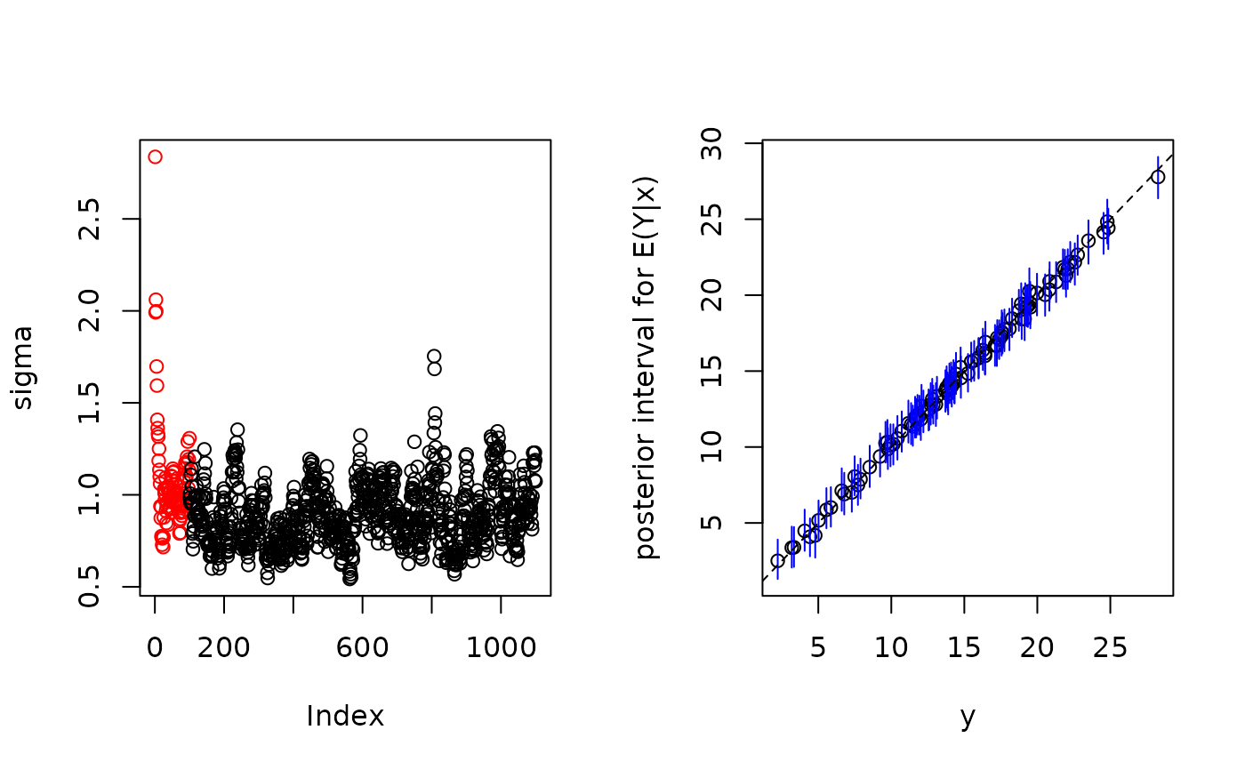
For continuous response fits, the plot method sets mfrow to c(1, 2) and makes two plots, unless sigma was held fixed, when it draws only the second. The first plot is the sequence of kept draws of \(\sigma\) including the burn-in draws. Initially these draws will decline as BART finds a good fit and then level off when the MCMC has burned in. The second plot has \(y\) on the horizontal axis and posterior intervals for the corresponding \(f(x)\) on the vertical axis. For binary response fits, only this second kind of plot is drawn, with the posterior median of \(P(Y = 1 \mid x)\) on the horizontal axis and its posterior interval on the vertical axis.
For print.bart, the fit itself (x), returned invisibly; the call and a short synopsis (family, chain/tree/burn counts, kept-draw count) print to the console as the side effect. A fit of several forests adds a short block of one line for each, its label, what the forest multiplies, a numeric column's mean and sd, and the sd the forest resolved to (for a numeric column, per sd of the column as it now stands), with a last line pointing to summary(), which gives the full block (see the sd argument of forest for what to read in it); a fit made with keepFits = FALSE prints the same block, from its labels and tree counts and, in place of each basis vector, a few numbers it keeps (element basis.columns: a numeric column's mean, sd, range and whether it is constant over the rows in the likelihood, a factor's levels). Such a fit still refuses predict at new rows, which needs the per-forest fits keepFits = FALSE dropped. A fit saved by dbarts 0.9-34 prints its call and then a note, as a message, that it cannot be read by this version and is to be refit; every other use of such a fit that needs its trees or sampler stops with that sentence.
References
Chipman, H., George, E., and McCulloch, R. (2010) BART: Bayesian additive regression trees. The Annals of Applied Statistics, 4(1), 266–298. doi:10.1214/09-AOAS285 .
Chipman, H., George, E., and McCulloch R. (2006) Bayesian Ensemble Learning. Advances in Neural Information Processing Systems 19, Scholkopf, Platt and Hoffman, Eds., MIT Press, Cambridge, MA, 265-272. https://www.rob-mcculloch.org
Friedman, J.H. (1991) Multivariate adaptive regression splines. The Annals of Statistics, 19, 1–67.
Calling extract
Call it as dbarts::extract. Other packages export a function named
extract: rstan, tidyr, terra, raster,
magrittr and R.utils. Whichever is attached last masks the
others, so a bare extract(fit, ...) may reach the wrong one. The
stan4bart package attaches dbarts, so it brings this name in.
Author
Hugh Chipman: hugh.chipman@gmail.com, Robert McCulloch: robert.mcculloch1@gmail.com, Vincent Dorie: vdorie@gmail.com.
See also
bart for the formula-first interface, further response families, and formula-term multi-forest models.
dbartsSampler's $predictForests for the same per-forest replay from a mutable sampler, which is what predict(type = "forest") reads and what extract(type = "forest") reports in sample.
dbarts-embedding and vignette("dbarts-as-a-component", package = "dbarts") for
using BART as one block of a sampler you write, rather than as the whole fit: these functions own
their own MCMC loop, while dbarts returns a
dbartsSampler that runs one sweep at a time.
Examples
## simulate data (example from Friedman MARS paper)
## y = f(x) + epsilon , epsilon ~ N(0, sigma)
## x consists of 10 variables, only first 5 matter
f <- function(x) {
10 * sin(pi * x[,1] * x[,2]) + 20 * (x[,3] - 0.5)^2 +
10 * x[,4] + 5 * x[,5]
}
set.seed(99)
sigma <- 1.0
n <- 100
x <- matrix(runif(n * 10), n, 10)
Ey <- f(x)
y <- rnorm(n, Ey, sigma)
## run BART
set.seed(99)
bartFit <- bartBT(x, y)
#> estimating the starting sigma by a dense linear regression on 100 rows and 10 columns; see 'sigest'
#>
#> Running BART with numeric y
#>
#> number of trees: 200
#> number of chains: 1, default number of threads 1
#> tree thinning rate: 1
#> Prior:
#> k prior fixed to 2.000000
#> degrees of freedom in sigma prior: 3.000000
#> quantile in sigma prior: 0.900000
#> scale in sigma prior: 0.002181
#> power and base for tree prior: 2.000000 0.950000
#> use quantiles for rule cut points: false
#> level fiber gibbs step: auto
#> proposal probabilities: birth/death 0.50, swap 0.10, change 0.40, perturb 0.00, rule_gibbs 0.00; birth 0.50; perturb window 1
#> data:
#> number of training observations: 100
#> number of test observations: 0
#> number of explanatory variables: 10
#> init sigma: 2.756573, curr sigma: 2.756573
#>
#> Cutoff rules c in x<=c vs x>c
#> Number of cutoffs: (var: number of possible c):
#> (1: 100) (2: 100) (3: 100) (4: 100) (5: 100)
#> (6: 100) (7: 100) (8: 100) (9: 100) (10: 100)
#>
#> Running mcmc loop:
#> iteration: 100 (of 1000)
#> iteration: 200 (of 1000)
#> iteration: 300 (of 1000)
#> iteration: 400 (of 1000)
#> iteration: 500 (of 1000)
#> iteration: 600 (of 1000)
#> iteration: 700 (of 1000)
#> iteration: 800 (of 1000)
#> iteration: 900 (of 1000)
#> iteration: 1000 (of 1000)
#> total seconds in loop: 0.121901
#>
#> Tree sizes, last iteration:
#> [1] 2 3 3 2 2 2 2 2 4 2 3 3 3 1 2 1 2 3
#> 2 2 4 2 2 3 3 2 2 2 2 3 2 2 2 1 3 3 2 2
#> 2 2 3 4 2 2 2 4 3 2 2 3 1 2 3 2 2 3 3 2
#> 3 2 2 2 2 3 2 2 3 2 2 2 2 2 2 2 2 3 2 2
#> 2 2 2 2 3 5 2 2 3 2 2 2 1 3 2 2 2 3 2 2
#> 1 2 5 1 3 3 3 4 2 2 2 2 3 2 2 2 2 2 2 1
#> 2 4 2 2 2 2 3 2 2 2 2 4 2 2 3 2 2 2 2 3
#> 2 3 2 2 2 2 2 1 2 4 4 3 2 4 4 3 2 1 2 3
#> 3 4 3 2 3 2 2 2 2 2 2 4 2 3 2 3 3 2 2 2
#> 3 2 2 3 2 2 2 4 4 2 3 1 3 2 2 2 1 3 2 4
#> 2 2
#>
#> Variable Usage, last iteration (var:count):
#> (1: 34) (2: 29) (3: 29) (4: 30) (5: 25)
#> (6: 25) (7: 36) (8: 21) (9: 28) (10: 16)
#>
#> DONE BART
#>
plot(bartFit)
 ## compare BART fit to linear matter and truth = Ey
lmFit <- lm(y ~ ., data.frame(x, y))
fitmat <- cbind(y, Ey, lmFit$fitted, bartFit$yhat.train.mean)
colnames(fitmat) <- c('y', 'Ey', 'lm', 'bart')
print(cor(fitmat))
#> y Ey lm bart
#> y 1.0000000 0.9847984 0.8841787 0.9984931
#> Ey 0.9847984 1.0000000 0.9009389 0.9886903
#> lm 0.8841787 0.9009389 1.0000000 0.8975062
#> bart 0.9984931 0.9886903 0.8975062 1.0000000
## fit with missing predictor values: every split rule learns a
## direction for NAs (MIA, always on; no argument selects it)
set.seed(1)
n <- 60L
x.na <- matrix(runif(n * 2), n, 2)
x.na[1:5, 1] <- NA
y.na <- x.na[,2] + rnorm(n, 0, 0.3)
y.na[is.na(x.na[,1])] <- y.na[is.na(x.na[,1])] + 2
fit.na <- dbarts(y.na ~ x.na, control = dbartsControl(
n.samples = 20L, n.burn = 20L, n.chains = 1L, n.threads = 1L),
n.trees = 20L)
samples.na <- fit.na$run()
## recipe: between-draws row subsetting on a latent family (e.g. principal
## stratification or mediation, where an outer Gibbs step redraws which rows
## belong to a stratum every iteration). $setActiveRows changes which rows
## are "in" the model from one run() to the next, without rebuilding the
## sampler and without losing any row's fitted value; see the "active" entry
## of \link{dbartsSampler-class} for the full semantics. Unlike zero case
## weights (gaussian, probit, ordinal and nbinom only), this also reaches
## logistic and aft samplers - and an emptied stratum is a legal all-zeros mask
## rather than a case the caller must special-case and skip.
set.seed(3)
n <- 120L
x.strat <- matrix(runif(n * 2), n, 2)
y.strat <- rbinom(n, 1L, plogis(2 * x.strat[,1] - 1))
sampler.strat <- dbarts(x.strat, y.strat, family = "probit",
control = dbartsControl(n.chains = 1L, n.threads = 1L,
updateState = FALSE),
n.trees = 20L)
stratum <- rbinom(n, 1L, 0.6) # this iteration's stratum membership
sampler.strat$setActiveRows(stratum)
draws.strat <- sampler.strat$run(20L, 20L)
## the next outer iteration redraws the stratum; even a stratum that empties
## out is accepted and runs, rather than needing to be skipped
stratum <- rep(0, n)
sampler.strat$setActiveRows(stratum)
draws.empty <- sampler.strat$run(0L, 5L)